Neural Network Zoo Prequel: Cells and Layers

Posted on

Cells

The Neural Network Zoo shows different types of cells and various layer connectivity styles, but it doesn’t really go into how each cell type works. A number of cell types I originally gave different colours to differentiate the networks more clearly, but I have since found out that these cells work more or less the same way, so you’ll find descriptions under the basic cell images.

A basic neural network cell, the type one would find in a regular feed forward architecture, is quite simple. The cell is connected to other neurons via weights, i.e. it can be connected to all the neurons in the previous layer. Each connection has its own weight, which is often just a random number at first. A weight can be negative, positive, very small, very big or zero. The value of each of the cells it’s connected to is multiplied by its respective connection weight. The resulting values are all added together. On top of this, a bias is also added. A bias can prevent a cell from getting stuck on outputting zero and it can speed up some operations, reducing the amount of neurons required to solve a problem. The bias is also a number, sometimes constant (often -1 or 1) and sometimes variable. This total sum is then passed through an activation function, the resulting value of which then becomes the value of the cell.

Convolutional cells are much like feed forward cells, except they’re typically connected to only a few neurons from the previous layer. They are often used to preserve spatial information, because they are connected not to a few random cells but to all cells in a certain proximity. This makes them practical for data with lots of localised information, such as images and sound waves (but mostly images). Deconvolutional cells are just the opposite: these tend to decode spatial information by being locally connected to the next layer. Both cells often have a lot of clones which are trained independently; each clone having it’s own weights but connected exactly the same way. These clones can be thought of as being located in separate networks which all have the same structure. Both are essentially the same as regular cells, but they are used differently.

Pooling and interpolating cells are frequently combined with convolutional cells. These cells are not really cells, more just raw operations. Pooling cells take in the incoming connections and decide which connection gets passed through. In images, this can be thought of as zooming out on a picture. You can no longer see all the pixels, and it has to learn which pixels to keep and which to discard. Interpolating cells perform the opposite operation: they take in some information and map it to more information. The extra information is made up, like if one where to zoom in on a small resolution picture. Interpolating cells are not the only reverse operation of pooling cells, but they are relatively common as they are fast and simple to implement. They are respectively connected much like convolutional and deconvolutional cells.

Mean and standard deviation cells (almost exclusively found in couples as probabilistic cells) are used to represent probability distributions. The mean is the average value and the standard deviation represents how far to deviate from this average (in both directions). For example, a probabilistic cell used for images could contain the information on how much red there is in a particular pixel. The mean would say for example 0.5, and the standard deviation 0.2. When sampling from these probabilistic cells, one would enter these values in a Gaussian random number generator, resulting in anything between 0.4 and 0.6 being quite likely results, with values further away from 0.5 being less and less likely (but still possible). They are often fully connected to either the previous or the next layer and they do not have biases.

Recurrent cells have connections not just in the realm of layers, but also over time. Each cell internally stores its previous value. They are updated just like basic cells, but with extra weights: connected to the previous values of the cells and most of the time also to all the cells in the same layer. These weights between the current value and the stored previous value work much like a volatile memory (like RAM), inheriting both properties of having a certain “state” and vanishing if not fed. Because the previous value is a value passed through an activation function, and each update passes this activated value along with the other weights through the activation function, information is continually lost. In fact, the retention rate is so low, that only four or five iterations later, almost all of the information is lost.

Long short term memory cells are used to combat the problem of the rapid information loss occurring in recurrent cells. LSTM cells are logic circuits, copied from how memory cells were designed for computers. Compared to RNN cells which store two states, LSTM cells store four: the current and last value of the output and the current and last values of the state of the “memory cell”. They have three “gates”: input, output, forget, and they also have just the regular input. Each of these gates has its own weight meaning that connecting to this type of cell entails setting up four weights (instead of just one). The gates function much like flow gates, not fence gates: they can let everything through, just a little bit, nothing, or, anything in between. This works by multiplying incoming information by a value ranging from 0 to 1, which is stored in this gate value. The input gate, then, determines how much of the input is allowed to be added to the cell value. The output gate determines how much of the output value can be seen by the rest of the network. The forget gate is not connected to the previous value of the output cell, but rather connected to the previous memory cell value. It determines how much of the last memory cell state to retain. Because it’s not connected to the output, much less information loss occurs, because no activation function is placed in the loop.

Gated recurrent units (cells) are a variation of LSTM cells. They too use gates to combat information loss, but do so with just 2 gates: update and reset. This makes them slightly less expressive but also slightly faster, as they use less connections everywhere. In essence there are two differences between LSTM cells and GRU cells: GRU cells do not have a hidden cell state protected by an output gate, and they combine the input and forget gate into a single update gate. The idea is that if you want to allow a lot of new information, you can probably forget some old information (and the other way around).

Layers

The most basic way of connecting neurons to form graphs is by connecting everything to absolutely everything. This is seen in Hopfield networks and Boltzmann machines. Of course, this means the number of connections grows exponentially, but the expressiveness is uncompromised. This is referred to as completely (or fully) connected.

After a while it was discovered that breaking the network up into distinct layers is a useful feature, where the definition of a layer is a set or group of neurons which are not connected to each other, but only to neurons from other group(s). This concept is for instance used in Restricted Boltzmann Machines. The idea of using layers is nowadays generalised for any number of layers and it can be found in almost all current architectures. This is (perhaps confusingly) also called fully connected or completely connected, because actually completely connected networks are quite uncommon.

Convolutionally connected layers are even more constrained than fully connected layers: we connect every neuron only to neurons in other groups that are close by. Images and sound waves contain a very high amount of information if used to feed directly one-to-one into a network (e.g. using one neuron per pixel). The idea of convolutional connections comes from the observation that spatial information is probably important to retain. It turned out that this is a good guess, as it’s used in many image and sound wave based neural network applications. This setup is however less expressive than fully connected layers. In essence it is a way of “importance” filtering, deciding which of the tightly grouped information packets are important; convolutional connections are great for dimensionality reduction. At what spatial distance neurons can still be connected depends on the implementation, but ranges higher than 4 or 5 neurons are rarely used. Note that “spatial” often refers to two-dimensional space, which is why most representations show three-dimensional sheets of neurons being connected; the connection range is applied in all dimensions.

Another option is of course to randomly connected neurons. This comes in two main variations as well: by allowing for some percentage of all possible connections, or to connect some percentage of neurons between layers. Random connections help to linearly reduce the performance of the network and can be useful in large networks where fully connected layers run into performance problems. A slightly more sparsely connected layer with slightly more neurons can perform better in some cases, especially where a lot of information needs to be stored but not as much information needs to be exchanged (a bit similar to the effectiveness of convolutionally connected layers, but then randomised). Very sparsely connected systems (1 or 2%) are also used, as seen in ELMs, ESNs and LSMs. Especially in the case of spiking networks this makes a lot of sense, because the more connections a neuron has, the less energy each weight will carry over, meaning less propagating and repeating patterns.

Time delayed connections are connections between neurons (often from the same layer, and even connected with themselves) that don’t get information from the previous layer, but from a layer from the past (previous iteration, mostly). This allows temporal (time, sequence or order) related information to be stored. These types of connections are often manually reset from time to time, to clear the “state” of the network. The key difference with regular connections is that these connections are continuously changing, even when the network isn’t being trained.

The following image shows some small sample networks of the types described above, and their connections. I use it when I get stuck on just exactly what is connected to what (which is particularly likely when working with LSTM or GRU cells):

Analyzing Six Deep Learning Tools for Music Generation

Posted on

As deep learning is gaining in popularity, creative applications are gaining traction as well. Looking at music generation through deep learning, new algorithms and songs are popping up on a weekly basis. In this post we will go over six major players in the field, and point out some difficult challenges these systems still face. GitHub links are provided for those who are interested in the technical details (or if you’re looking to generate some music of your own).

Magenta

Magenta is Google’s open source deep learning music project. They aim to use machine learning to generate compelling music. The project went open source in June 2016 and currently implements a regular RNN and two LSTM’s.
GitHub: https://github.com/tensorflow/magenta
Great, because: It can handle any monophonic midi file. The documentation is good, so it’s relatively easy to set-up. The team is actively improving the models and adding functionality. For every model Magenta has provided a training bundle that is trained on thousands of midi files. You can start generating new midi files right away using these pre-trained models.
Challenges: At this point, Magenta can only generate a single stream of notes. Efforts have been made to combine the generated melodies with drums and guitars – but based on human input, as of yet. Once a model that can process polyphonic music has been trained, it could start to create harmonies (or at least multiple streams of notes). This would indeed be a mighty step on their quest for the generation of some compelling music.
Sounds like: The piece below is generated by Magenta from the 8th note onward. Here they use their attention model with the provided pre-trained bundle.

DeepJazz

The result of a thirty-six-hour hackathon by Ji-Sung Kim. It uses a two layer LSTM that learns from a midi file as its input source. DeepJazz has received quite some news coverage in the first six months of its existence.
GitHub: https://github.com/jisungk/deepjazz
Great, because: Can create some jazz by being trained on a single midi file. The project itself is also compelling proof that creating a working computational music prototype using deep learning techniques can be a matter of hours thanks to libraries like Keras, Theano & Tensorflow.
Challenges: While it can handle chords, it converts the jazz midi to a single pitch and single instrument. It would take a few more post-processing steps for the deep learning created melodies to sound more like human created jazz music.
Sounds like: The following piece is generated after 128 epochs (i.e. the training set consisting of a single midi file has cycled through the model that many times).

BachBot

A research project by Feynman Liang at Cambridge University,  also using an LSTM. This time it is used to train itself on Bach chorales. It’s goal is to generate and harmonize chorales indistinguishable from Bach’s own work. The website offers a test where one can listen to two streams and guess which one is an actual composition by Bach.
GitHub: https://github.com/feynmanliang/bachbot/
Great, because: Research found that people have a hard time distinguishing generated Bach from the real stuff. Also, this is one of the best efforts in handling polyphonic music as the algorithm can handle up to four voices.
Challenges: BachBot works best if one or more of the voices are fixed. Otherwise the algorithm just generates wandering chorales.The algorithm could be used to add chorales to a generated melody.
Sounds like: In the below example the notes for “Twinkle Twinkle Little Star” were fixed, with the chorales generated.

FlowMachines

In the picturesque city of Paris, a research team is working on a system that can help to keep an artist in a creative flow. Their system can generate leadsheets based on the style of a composer in a database filled with about 13000 sheets. Markov constraints are used here as neural network technique.
GitHub: not open source.
Great, because: The system has composed the first AI pop-songs.
Challenges: Producing pop songs from a generated leadsheet to these pop songs is not simply done at the click of a button – it still requires a well-skilled musician to create a compelling song like in the example below. Reducing the difficulty of these steps with the help of deep learning is still an open challenge.
Sounds like: The song is composed by the FlowMachines AI. In order to do so, the musician chose the “Beatles” style, and generated melody and harmony. Note the rest of the score (production, mixing, and assigning audio pieces to the notes) was produces by human composer.

WaveNet

Researchers at Google’s DeepMind have created Wavenet. Wavenet is based on Convolutional Neural Networks, the deep learning technique that works very well in image classification and generation in the past few years. Their most promising purpose is to enhance text-to-speech applications by generating a more natural flow in vocal sound. However, their method can also be applied to music as both the input and output consists of raw audio.
GitHub: WaveNet’s code is not open source, but others have implemented it based on DeepMind’s documentation. For example: https://github.com/ibab/tensorflow-wavenet
Great, because: It uses raw audio as input. Therefore it can generate any kind of instrument, and even any kind of sound. It will be interesting to see what this technique is capable of once trained on hours of music.
Challenges: The algorithm is computationally expensive. It takes minutes to train on a second of sound. Some have started to create a faster version. Another researcher working for Google, Sageev Oore from the Magenta project, has written a blog post where he describes what can be learned from the musical output of Wavenet. One of his conclusions is that the algorithm can produce piano notes without a beginning, making them unplayable on a real piano. Interestingly, Wavenet can extend the current library of sounds that a piano can create and produce a new form of piano music – perhaps the next step in (generated) music.
Sounds like: Trained on a dataset of piano music results in the following ten seconds of sound:

GRUV

A Stanford research project that, similar to Wavenet, also tries to use audio waveforms as input, but with an LSTM’s and GRU’s rather than CNN’s. They have showed their proof of concept to the world in June 2015.
GitHub: https://github.com/MattVitelli/GRUV
Great, because: The Stanford researchers were one of the first to show how to generate sounds with an LSTM using raw waveforms as input.
Challenges: The demonstration they provide seems over-fitted on a particular song, due to the small training corpus and the sheer amount of layers of the NN. The researchers themselves did not have the time nor computational power to experiment further with this. Fortunately, this void is starting to get filled by researchers from WaveNet and other enthusiasts. Jakub Fiala has used this code to generate an interesting amen drum break, see this blog post.
Sounds like: The tool trained on a variety of Madeon songs, resulted in the below sample. Until 1:10 is an excerpt of the creation after 100 up to 1000 iterations, after that is a mash-up of their best generated pieces. This excerpt is a recording of this video.

Notes VS Waves

The described deep learning music applications can be divided into two categories based on the input method. Magenta, DeepJazz, BachBot, and FlowMachines all use input in the form of note sequences, while GRUV and Wavenet use raw audio.

Input type: Note sequences Raw audio
Computational complexity Low (minutes – few hours) High (few hours – days)
Editable result Yes, can be imported in music production software No, waveform itself has to be edited
Musical complexity As complex as a single song from the corpus As complex as the combination of the entire corpus

Can we call out a clear winner? In my opinion: no. Each has different applications and these methods can coexist until generating compelling music with raw audio becomes so fast that there is simply no point in doing it yourself.

Music will be easier to create by people who are assisted by an AI that can suggest a melody or harmony. However, these people still need to be musicians (for now). The moment it is possible to train a deep learning algorithm on your entire Spotify history in raw audio form, and generate new songs, everyone can be a musician.

Image classification and generation has been improved with neural network techniques, reaching higher benchmark scores than ever before, mostly thanks to the speed at which huge sets of pixels can be trained. For audio the overarching question is: when will raw audio overtake notes as the pixel of music?


Did you miss anything, or do you have any other feedback? Comments are greatly appreciated. At the Asimov Institute we do deep learning research and development, so be sure to follow us on Twitter for future updates and posts!  In this post we did no go into the technical details, but if you’re new to deep learning or unfamiliar with a method, I refer you to one of our previous posts on neural networks.

We are currently working on generating electronic dance music using deep learning. If you want to share your ideas on this, or have some interesting data to show, please send a message to frankbrinkkemper@gmail.com. Thank you for reading!

The Neural Network Zoo

Posted on

With new neural network architectures popping up every now and then, it’s hard to keep track of them all. Knowing all the abbreviations being thrown around (DCIGN, BiLSTM, DCGAN, anyone?) can be a bit overwhelming at first.

So I decided to compose a cheat sheet containing many of those architectures. Most of these are neural networks, some are completely different beasts. Though all of these architectures are presented as novel and unique, when I drew the node structures… their underlying relations started to make more sense.

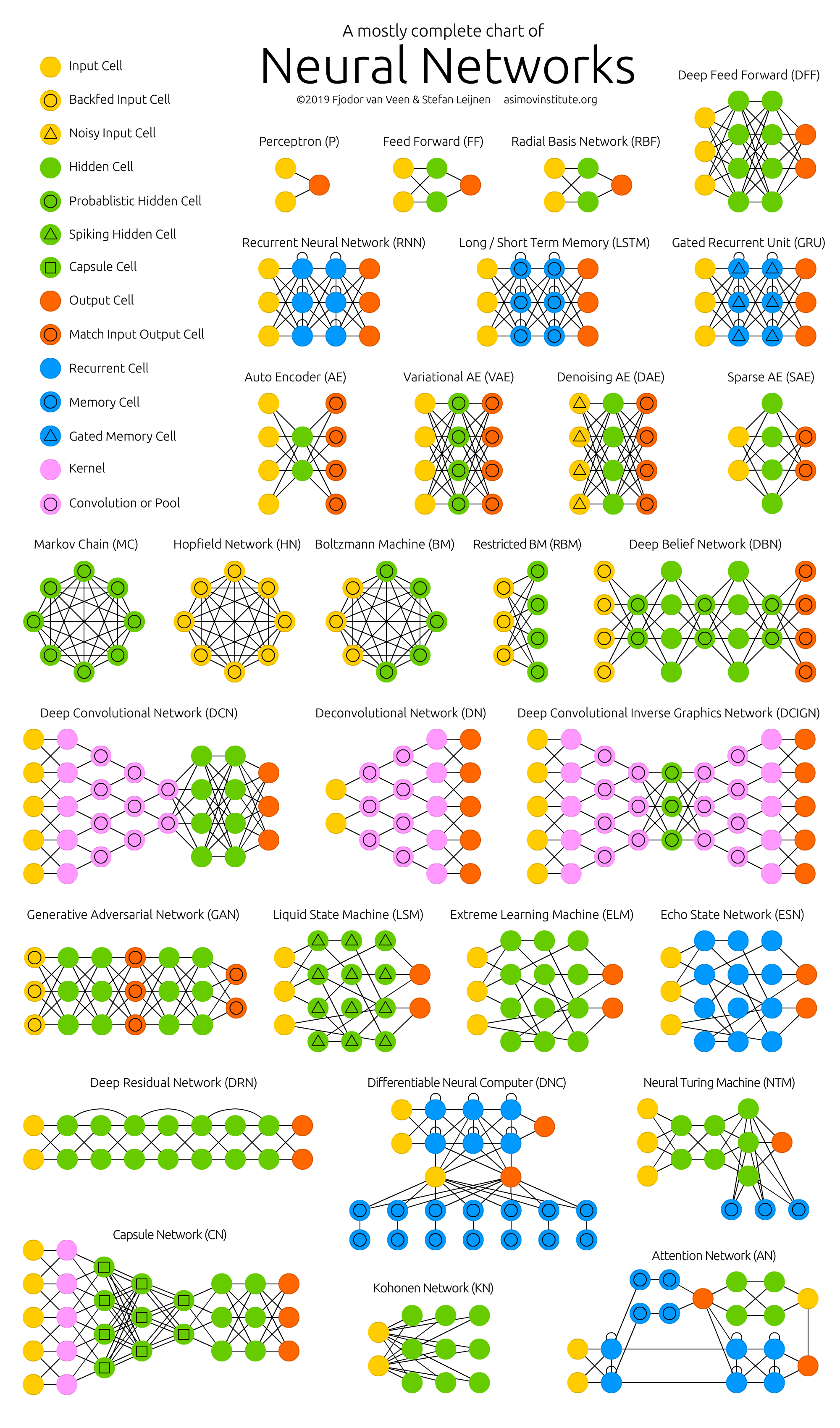
The Neural Network Zoo (download or get the poster).

One problem with drawing them as node maps: it doesn’t really show how they’re used. For example, variational autoencoders (VAE) may look just like autoencoders (AE), but the training process is actually quite different. The use-cases for trained networks differ even more, because VAEs are generators, where you insert noise to get a new sample. AEs, simply map whatever they get as input to the closest training sample they “remember”. I should add that this overview is in no way clarifying how each of the different node types work internally (but that’s a topic for another day).

It should be noted that while most of the abbreviations used are generally accepted, not all of them are. RNNs sometimes refer to recursive neural networks, but most of the time they refer to recurrent neural networks. That’s not the end of it though, in many places you’ll find RNN used as placeholder for any recurrent architecture, including LSTMs, GRUs and even the bidirectional variants. AEs suffer from a similar problem from time to time, where VAEs and DAEs and the like are called simply AEs. Many abbreviations also vary in the amount of “N”s to add at the end, because you could call it a convolutional neural network but also simply a convolutional network (resulting in CNN or CN).

Composing a complete list is practically impossible, as new architectures are invented all the time. Even if published it can still be quite challenging to find them even if you’re looking for them, or sometimes you just overlook some. So while this list may provide you with some insights into the world of AI, please, by no means take this list for being comprehensive; especially if you read this post long after it was written.

For each of the architectures depicted in the picture, I wrote a very, very brief description. You may find some of these to be useful if you’re quite familiar with some architectures, but you aren’t familiar with a particular one.


Feed forward neural networks (FF or FFNN) and perceptrons (P) are very straight forward, they feed information from the front to the back (input and output, respectively). Neural networks are often described as having layers, where each layer consists of either input, hidden or output cells in parallel. A layer alone never has connections and in general two adjacent layers are fully connected (every neuron form one layer to every neuron to another layer). The simplest somewhat practical network has two input cells and one output cell, which can be used to model logic gates. One usually trains FFNNs through back-propagation, giving the network paired datasets of “what goes in” and “what we want to have coming out”. This is called supervised learning, as opposed to unsupervised learning where we only give it input and let the network fill in the blanks. The error being back-propagated is often some variation of the difference between the input and the output (like MSE or just the linear difference). Given that the network has enough hidden neurons, it can theoretically always model the relationship between the input and output. Practically their use is a lot more limited but they are popularly combined with other networks to form new networks.

Rosenblatt, Frank. “The perceptron: a probabilistic model for information storage and organization in the brain.” Psychological review 65.6 (1958): 386.
Original Paper PDF


Radial basis function (RBF) networks are FFNNs with radial basis functions as activation functions. There’s nothing more to it. Doesn’t mean they don’t have their uses, but most FFNNs with other activation functions don’t get their own name. This mostly has to do with inventing them at the right time.

Broomhead, David S., and David Lowe. Radial basis functions, multi-variable functional interpolation and adaptive networks. No. RSRE-MEMO-4148. ROYAL SIGNALS AND RADAR ESTABLISHMENT MALVERN (UNITED KINGDOM), 1988.
Original Paper PDF


Recurrent neural networks (RNN) are FFNNs with a time twist: they are not stateless; they have connections between passes, connections through time. Neurons are fed information not just from the previous layer but also from themselves from the previous pass. This means that the order in which you feed the input and train the network matters: feeding it “milk” and then “cookies” may yield different results compared to feeding it “cookies” and then “milk”. One big problem with RNNs is the vanishing (or exploding) gradient problem where, depending on the activation functions used, information rapidly gets lost over time, just like very deep FFNNs lose information in depth. Intuitively this wouldn’t be much of a problem because these are just weights and not neuron states, but the weights through time is actually where the information from the past is stored; if the weight reaches a value of 0 or 1 000 000, the previous state won’t be very informative. RNNs can in principle be used in many fields as most forms of data that don’t actually have a timeline (i.e. unlike sound or video) can be represented as a sequence. A picture or a string of text can be fed one pixel or character at a time, so the time dependent weights are used for what came before in the sequence, not actually from what happened x seconds before. In general, recurrent networks are a good choice for advancing or completing information, such as autocompletion.

Elman, Jeffrey L. “Finding structure in time.” Cognitive science 14.2 (1990): 179-211.
Original Paper PDF


Long / short term memory (LSTM) networks try to combat the vanishing / exploding gradient problem by introducing gates and an explicitly defined memory cell. These are inspired mostly by circuitry, not so much biology. Each neuron has a memory cell and three gates: input, output and forget. The function of these gates is to safeguard the information by stopping or allowing the flow of it. The input gate determines how much of the information from the previous layer gets stored in the cell. The output layer takes the job on the other end and determines how much of the next layer gets to know about the state of this cell. The forget gate seems like an odd inclusion at first but sometimes it’s good to forget: if it’s learning a book and a new chapter begins, it may be necessary for the network to forget some characters from the previous chapter. LSTMs have been shown to be able to learn complex sequences, such as writing like Shakespeare or composing primitive music. Note that each of these gates has a weight to a cell in the previous neuron, so they typically require more resources to run.

Hochreiter, Sepp, and Jürgen Schmidhuber. “Long short-term memory.” Neural computation 9.8 (1997): 1735-1780.
Original Paper PDF


Gated recurrent units (GRU) are a slight variation on LSTMs. They have one less gate and are wired slightly differently: instead of an input, output and a forget gate, they have an update gate. This update gate determines both how much information to keep from the last state and how much information to let in from the previous layer. The reset gate functions much like the forget gate of an LSTM but it’s located slightly differently. They always send out their full state, they don’t have an output gate. In most cases, they function very similarly to LSTMs, with the biggest difference being that GRUs are slightly faster and easier to run (but also slightly less expressive). In practice these tend to cancel each other out, as you need a bigger network to regain some expressiveness which then in turn cancels out the performance benefits. In some cases where the extra expressiveness is not needed, GRUs can outperform LSTMs.

Chung, Junyoung, et al. “Empirical evaluation of gated recurrent neural networks on sequence modeling.” arXiv preprint arXiv:1412.3555 (2014).
Original Paper PDF


Bidirectional recurrent neural networks, bidirectional long / short term memory networks and bidirectional gated recurrent units (BiRNN, BiLSTM and BiGRU respectively) are not shown on the chart because they look exactly the same as their unidirectional counterparts. The difference is that these networks are not just connected to the past, but also to the future. As an example, unidirectional LSTMs might be trained to predict the word “fish” by being fed the letters one by one, where the recurrent connections through time remember the last value. A BiLSTM would also be fed the next letter in the sequence on the backward pass, giving it access to future information. This trains the network to fill in gaps instead of advancing information, so instead of expanding an image on the edge, it could fill a hole in the middle of an image.

Schuster, Mike, and Kuldip K. Paliwal. “Bidirectional recurrent neural networks.” IEEE Transactions on Signal Processing 45.11 (1997): 2673-2681.
Original Paper PDF


Autoencoders (AE) are somewhat similar to FFNNs as AEs are more like a different use of FFNNs than a fundamentally different architecture. The basic idea behind autoencoders is to encode information (as in compress, not encrypt) automatically, hence the name. The entire network always resembles an hourglass like shape, with smaller hidden layers than the input and output layers. AEs are also always symmetrical around the middle layer(s) (one or two depending on an even or odd amount of layers). The smallest layer(s) is|are almost always in the middle, the place where the information is most compressed (the chokepoint of the network). Everything up to the middle is called the encoding part, everything after the middle the decoding and the middle (surprise) the code. One can train them using backpropagation by feeding input and setting the error to be the difference between the input and what came out. AEs can be built symmetrically when it comes to weights as well, so the encoding weights are the same as the decoding weights.

Bourlard, Hervé, and Yves Kamp. “Auto-association by multilayer perceptrons and singular value decomposition.” Biological cybernetics 59.4-5 (1988): 291-294.
Original Paper PDF


Variational autoencoders (VAE) have the same architecture as AEs but are “taught” something else: an approximated probability distribution of the input samples. It’s a bit back to the roots as they are bit more closely related to BMs and RBMs. They do however rely on Bayesian mathematics regarding probabilistic inference and independence, as well as a re-parametrisation trick to achieve this different representation. The inference and independence parts make sense intuitively, but they rely on somewhat complex mathematics. The basics come down to this: take influence into account. If one thing happens in one place and something else happens somewhere else, they are not necessarily related. If they are not related, then the error propagation should consider that. This is a useful approach because neural networks are large graphs (in a way), so it helps if you can rule out influence from some nodes to other nodes as you dive into deeper layers.

Kingma, Diederik P., and Max Welling. “Auto-encoding variational bayes.” arXiv preprint arXiv:1312.6114 (2013).
Original Paper PDF


Denoising autoencoders (DAE) are AEs where we don’t feed just the input data, but we feed the input data with noise (like making an image more grainy). We compute the error the same way though, so the output of the network is compared to the original input without noise. This encourages the network not to learn details but broader features, as learning smaller features often turns out to be “wrong” due to it constantly changing with noise.

Vincent, Pascal, et al. “Extracting and composing robust features with denoising autoencoders.” Proceedings of the 25th international conference on Machine learning. ACM, 2008.
Original Paper PDF


Sparse autoencoders (SAE) are in a way the opposite of AEs. Instead of teaching a network to represent a bunch of information in less “space” or nodes, we try to encode information in more space. So instead of the network converging in the middle and then expanding back to the input size, we blow up the middle. These types of networks can be used to extract many small features from a dataset. If one were to train a SAE the same way as an AE, you would in almost all cases end up with a pretty useless identity network (as in what comes in is what comes out, without any transformation or decomposition). To prevent this, instead of feeding back the input, we feed back the input plus a sparsity driver. This sparsity driver can take the form of a threshold filter, where only a certain error is passed back and trained, the other error will be “irrelevant” for that pass and set to zero. In a way this resembles spiking neural networks, where not all neurons fire all the time (and points are scored for biological plausibility).

Marc’Aurelio Ranzato, Christopher Poultney, Sumit Chopra, and Yann LeCun. “Efficient learning of sparse representations with an energy-based model.” Proceedings of NIPS. 2007.
Original Paper PDF


Markov chains (MC or discrete time Markov Chain, DTMC) are kind of the predecessors to BMs and HNs. They can be understood as follows: from this node where I am now, what are the odds of me going to any of my neighbouring nodes? They are memoryless (i.e. Markov Property) which means that every state you end up in depends completely on the previous state. While not really a neural network, they do resemble neural networks and form the theoretical basis for BMs and HNs. MC aren’t always considered neural networks, as goes for BMs, RBMs and HNs. Markov chains aren’t always fully connected either.

Hayes, Brian. “First links in the Markov chain.” American Scientist 101.2 (2013): 252.
Original Paper PDF


A Hopfield network (HN) is a network where every neuron is connected to every other neuron; it is a completely entangled plate of spaghetti as even all the nodes function as everything. Each node is input before training, then hidden during training and output afterwards. The networks are trained by setting the value of the neurons to the desired pattern after which the weights can be computed. The weights do not change after this. Once trained for one or more patterns, the network will always converge to one of the learned patterns because the network is only stable in those states. Note that it does not always conform to the desired state (it’s not a magic black box sadly). It stabilises in part due to the total “energy” or “temperature” of the network being reduced incrementally during training. Each neuron has an activation threshold which scales to this temperature, which if surpassed by summing the input causes the neuron to take the form of one of two states (usually -1 or 1, sometimes 0 or 1). Updating the network can be done synchronously or more commonly one by one. If updated one by one, a fair random sequence is created to organise which cells update in what order (fair random being all options (n) occurring exactly once every n items). This is so you can tell when the network is stable (done converging), once every cell has been updated and none of them changed, the network is stable (annealed). These networks are often called associative memory because the converge to the most similar state as the input; if humans see half a table we can image the other half, this network will converge to a table if presented with half noise and half a table.

Hopfield, John J. “Neural networks and physical systems with emergent collective computational abilities.” Proceedings of the national academy of sciences 79.8 (1982): 2554-2558.
Original Paper PDF


Boltzmann machines (BM) are a lot like HNs, but: some neurons are marked as input neurons and others remain “hidden”. The input neurons become output neurons at the end of a full network update. It starts with random weights and learns through back-propagation, or more recently through contrastive divergence (a Markov chain is used to determine the gradients between two informational gains). Compared to a HN, the neurons mostly have binary activation patterns. As hinted by being trained by MCs, BMs are stochastic networks. The training and running process of a BM is fairly similar to a HN: one sets the input neurons to certain clamped values after which the network is set free (it doesn’t get a sock). While free the cells can get any value and we repetitively go back and forth between the input and hidden neurons. The activation is controlled by a global temperature value, which if lowered lowers the energy of the cells. This lower energy causes their activation patterns to stabilise. The network reaches an equilibrium given the right temperature.

Hinton, Geoffrey E., and Terrence J. Sejnowski. “Learning and releaming in Boltzmann machines.” Parallel distributed processing: Explorations in the microstructure of cognition 1 (1986): 282-317.
Original Paper PDF


Restricted Boltzmann machines (RBM) are remarkably similar to BMs (surprise) and therefore also similar to HNs. The biggest difference between BMs and RBMs is that RBMs are a better usable because they are more restricted. They don’t trigger-happily connect every neuron to every other neuron but only connect every different group of neurons to every other group, so no input neurons are directly connected to other input neurons and no hidden to hidden connections are made either. RBMs can be trained like FFNNs with a twist: instead of passing data forward and then back-propagating, you forward pass the data and then backward pass the data (back to the first layer). After that you train with forward-and-back-propagation.

Smolensky, Paul. Information processing in dynamical systems: Foundations of harmony theory. No. CU-CS-321-86. COLORADO UNIV AT BOULDER DEPT OF COMPUTER SCIENCE, 1986.
Original Paper PDF


Deep belief networks (DBN) is the name given to stacked architectures of mostly RBMs or VAEs. These networks have been shown to be effectively trainable stack by stack, where each AE or RBM only has to learn to encode the previous network. This technique is also known as greedy training, where greedy means making locally optimal solutions to get to a decent but possibly not optimal answer. DBNs can be trained through contrastive divergence or back-propagation and learn to represent the data as a probabilistic model, just like regular RBMs or VAEs. Once trained or converged to a (more) stable state through unsupervised learning, the model can be used to generate new data. If trained with contrastive divergence, it can even classify existing data because the neurons have been taught to look for different features.

Bengio, Yoshua, et al. “Greedy layer-wise training of deep networks.” Advances in neural information processing systems 19 (2007): 153.
Original Paper PDF


Convolutional neural networks (CNN or deep convolutional neural networks, DCNN) are quite different from most other networks. They are primarily used for image processing but can also be used for other types of input such as as audio. A typical use case for CNNs is where you feed the network images and the network classifies the data, e.g. it outputs “cat” if you give it a cat picture and “dog” when you give it a dog picture. CNNs tend to start with an input “scanner” which is not intended to parse all the training data at once. For example, to input an image of 200 x 200 pixels, you wouldn’t want a layer with 40 000 nodes. Rather, you create a scanning input layer of say 20 x 20 which you feed the first 20 x 20 pixels of the image (usually starting in the upper left corner). Once you passed that input (and possibly use it for training) you feed it the next 20 x 20 pixels: you move the scanner one pixel to the right. Note that one wouldn’t move the input 20 pixels (or whatever scanner width) over, you’re not dissecting the image into blocks of 20 x 20, but rather you’re crawling over it. This input data is then fed through convolutional layers instead of normal layers, where not all nodes are connected to all nodes. Each node only concerns itself with close neighbouring cells (how close depends on the implementation, but usually not more than a few). These convolutional layers also tend to shrink as they become deeper, mostly by easily divisible factors of the input (so 20 would probably go to a layer of 10 followed by a layer of 5). Powers of two are very commonly used here, as they can be divided cleanly and completely by definition: 32, 16, 8, 4, 2, 1. Besides these convolutional layers, they also often feature pooling layers. Pooling is a way to filter out details: a commonly found pooling technique is max pooling, where we take say 2 x 2 pixels and pass on the pixel with the most amount of red. To apply CNNs for audio, you basically feed the input audio waves and inch over the length of the clip, segment by segment. Real world implementations of CNNs often glue an FFNN to the end to further process the data, which allows for highly non-linear abstractions. These networks are called DCNNs but the names and abbreviations between these two are often used interchangeably.

LeCun, Yann, et al. “Gradient-based learning applied to document recognition.” Proceedings of the IEEE 86.11 (1998): 2278-2324.
Original Paper PDF


Deconvolutional networks (DN), also called inverse graphics networks (IGNs), are reversed convolutional neural networks. Imagine feeding a network the word “cat” and training it to produce cat-like pictures, by comparing what it generates to real pictures of cats. DNNs can be combined with FFNNs just like regular CNNs, but this is about the point where the line is drawn with coming up with new abbreviations. They may be referenced as deep deconvolutional neural networks, but you could argue that when you stick FFNNs to the back and the front of DNNs that you have yet another architecture which deserves a new name. Note that in most applications one wouldn’t actually feed text-like input to the network, more likely a binary classification input vector. Think <0, 1> being cat, <1, 0> being dog and <1, 1> being cat and dog. The pooling layers commonly found in CNNs are often replaced with similar inverse operations, mainly interpolation and extrapolation with biased assumptions (if a pooling layer uses max pooling, you can invent exclusively lower new data when reversing it).

Zeiler, Matthew D., et al. “Deconvolutional networks.” Computer Vision and Pattern Recognition (CVPR), 2010 IEEE Conference on. IEEE, 2010.
Original Paper PDF


Deep convolutional inverse graphics networks (DCIGN) have a somewhat misleading name, as they are actually VAEs but with CNNs and DNNs for the respective encoders and decoders. These networks attempt to model “features” in the encoding as probabilities, so that it can learn to produce a picture with a cat and a dog together, having only ever seen one of the two in separate pictures. Similarly, you could feed it a picture of a cat with your neighbours’ annoying dog on it, and ask it to remove the dog, without ever having done such an operation. Demo’s have shown that these networks can also learn to model complex transformations on images, such as changing the source of light or the rotation of a 3D object. These networks tend to be trained with back-propagation.

Kulkarni, Tejas D., et al. “Deep convolutional inverse graphics network.” Advances in Neural Information Processing Systems. 2015.
Original Paper PDF


Generative adversarial networks (GAN) are from a different breed of networks, they are twins: two networks working together. GANs consist of any two networks (although often a combination of FFs and CNNs), with one tasked to generate content and the other has to judge content. The discriminating network receives either training data or generated content from the generative network. How well the discriminating network was able to correctly predict the data source is then used as part of the error for the generating network. This creates a form of competition where the discriminator is getting better at distinguishing real data from generated data and the generator is learning to become less predictable to the discriminator. This works well in part because even quite complex noise-like patterns are eventually predictable but generated content similar in features to the input data is harder to learn to distinguish. GANs can be quite difficult to train, as you don’t just have to train two networks (either of which can pose it’s own problems) but their dynamics need to be balanced as well. If prediction or generation becomes to good compared to the other, a GAN won’t converge as there is intrinsic divergence.

Goodfellow, Ian, et al. “Generative adversarial nets.” Advances in Neural Information Processing Systems (2014).
Original Paper PDF


Liquid state machines (LSM) are similar soups, looking a lot like ESNs. The real difference is that LSMs are a type of spiking neural networks: sigmoid activations are replaced with threshold functions and each neuron is also an accumulating memory cell. So when updating a neuron, the value is not set to the sum of the neighbours, but rather added to itself. Once the threshold is reached, it releases its’ energy to other neurons. This creates a spiking like pattern, where nothing happens for a while until a threshold is suddenly reached.

Maass, Wolfgang, Thomas Natschläger, and Henry Markram. “Real-time computing without stable states: A new framework for neural computation based on perturbations.” Neural computation 14.11 (2002): 2531-2560.
Original Paper PDF


Extreme learning machines (ELM) are basically FFNNs but with random connections. They look very similar to LSMs and ESNs, but they are not recurrent nor spiking. They also do not use backpropagation. Instead, they start with random weights and train the weights in a single step according to the least-squares fit (lowest error across all functions). This results in a much less expressive network but it’s also much faster than backpropagation.

Huang, Guang-Bin, et al. “Extreme learning machine: Theory and applications.” Neurocomputing 70.1-3 (2006): 489-501.
Original Paper PDF


Echo state networks (ESN) are yet another different type of (recurrent) network. This one sets itself apart from others by having random connections between the neurons (i.e. not organised into neat sets of layers), and they are trained differently. Instead of feeding input and back-propagating the error, we feed the input, forward it and update the neurons for a while, and observe the output over time. The input and the output layers have a slightly unconventional role as the input layer is used to prime the network and the output layer acts as an observer of the activation patterns that unfold over time. During training, only the connections between the observer and the (soup of) hidden units are changed.

Jaeger, Herbert, and Harald Haas. “Harnessing nonlinearity: Predicting chaotic systems and saving energy in wireless communication.” science 304.5667 (2004): 78-80.
Original Paper PDF


Deep residual networks (DRN) are very deep FFNNs with extra connections passing input from one layer to a later layer (often 2 to 5 layers) as well as the next layer. Instead of trying to find a solution for mapping some input to some output across say 5 layers, the network is enforced to learn to map some input to some output + some input. Basically, it adds an identity to the solution, carrying the older input over and serving it freshly to a later layer. It has been shown that these networks are very effective at learning patterns up to 150 layers deep, much more than the regular 2 to 5 layers one could expect to train. However, it has been proven that these networks are in essence just RNNs without the explicit time based construction and they’re often compared to LSTMs without gates.

He, Kaiming, et al. “Deep residual learning for image recognition.” arXiv preprint arXiv:1512.03385 (2015).
Original Paper PDF


Neural Turing machines (NTM) can be understood as an abstraction of LSTMs and an attempt to un-black-box neural networks (and give us some insight in what is going on in there). Instead of coding a memory cell directly into a neuron, the memory is separated. It’s an attempt to combine the efficiency and permanency of regular digital storage and the efficiency and expressive power of neural networks. The idea is to have a content-addressable memory bank and a neural network that can read and write from it. The “Turing” in Neural Turing Machines comes from them being Turing complete: the ability to read and write and change state based on what it reads means it can represent anything a Universal Turing Machine can represent.

Graves, Alex, Greg Wayne, and Ivo Danihelka. “Neural turing machines.” arXiv preprint arXiv:1410.5401 (2014).
Original Paper PDF


Differentiable Neural Computers (DNC) are enhanced Neural Turing Machines with scalable memory, inspired by how memories are stored by the human hippocampus. The idea is to take the classical Von Neumann computer architecture and replace the CPU with an RNN, which learns when and what to read from the RAM. Besides having a large bank of numbers as memory (which may be resized without retraining the RNN). The DNC also has three attention mechanisms. These mechanisms allow the RNN to query the similarity of a bit of input to the memory’s entries, the temporal relationship between any two entries in memory, and whether a memory entry was recently updated – which makes it less likely to be overwritten when there’s no empty memory available.

Graves, Alex, et al. “Hybrid computing using a neural network with dynamic external memory.” Nature 538 (2016): 471-476.
Original Paper PDF


Capsule Networks (CapsNet) are biology inspired alternatives to pooling, where neurons are connected with multiple weights (a vector) instead of just one weight (a scalar). This allows neurons to transfer more information than simply which feature was detected, such as where a feature is in the picture or what colour and orientation it has. The learning process involves a local form of Hebbian learning that values correct predictions of output in the next layer.

Sabour, Sara, Frosst, Nicholas, and Hinton, G. E. “Dynamic Routing Between Capsules.” In Advances in neural information processing systems (2017): 3856-3866.
Original Paper PDF


Kohonen networks (KN, also self organising (feature) map, SOM, SOFM) utilise competitive learning to classify data without supervision. Input is presented to the network, after which the network assesses which of its neurons most closely match that input. These neurons are then adjusted to match the input even better, dragging along their neighbours in the process. How much the neighbours are moved depends on the distance of the neighbours to the best matching units.

Kohonen, Teuvo. “Self-organized formation of topologically correct feature maps.” Biological cybernetics 43.1 (1982): 59-69.
Original Paper PDF


Attention networks (AN) can be considered a class of networks, which includes the Transformer architecture. They use an attention mechanism to combat information decay by separately storing previous network states and switching attention between the states. The hidden states of each iteration in the encoding layers are stored in memory cells. The decoding layers are connected to the encoding layers, but it also receives data from the memory cells filtered by an attention context. This filtering step adds context for the decoding layers stressing the importance of particular features. The attention network producing this context is trained using the error signal from the output of decoding layer. Moreover, the attention context can be visualized giving valuable insight into which input features correspond with what output features.

Jaderberg, Max, et al. “Spatial Transformer Networks.” In Advances in neural information processing systems (2015): 2017-2025.
Original Paper PDF


Follow us on twitter for future updates and posts. We welcome comments and feedback, and thank you for reading!

[Update 22 April 2019] Included Capsule Networks, Differentiable Neural Computers and Attention Networks to the Neural Network Zoo; Support Vector Machines are removed; updated links to original articles. The previous version of this post can be found here .

Van Veen, F. & Leijnen, S. (2019). The Neural Network Zoo. Retrieved from https://www.asimovinstitute.org/neural-network-zoo

A Quick Guide to Installing TensorFlow on mac OS

Posted on

TL;DR: paste all the commands in your terminal in order of appearance; skip packages you already have (but update them).

Before we begin: make sure you have at least 50GB of free disk space and that your device isn’t running on battery power. We are going to run neural networks; just like the giant network in your brain it eats everything. Power, memory, time and even hard drives. It’s also good practice to make sure that your computer is properly cooled (all the vents have room to breathe). Your ambient room temperature shouldn’t be exceptionally high either (38C or 100F).

One day we might see a new software package or technology that you can install without dependancies and just a single command. Today is not that day, as TensorFlow has a spiderweb of used frameworks and libraries. But no matter, we simply install them one by one. For each library we install, you should check if you have it installed already. If you’re not sure it’s installed normally, you can opt to reinstall it or change the installation. In either case you should make sure you upgrade the package (get the latest version).

Some of the following commands require sudo (which means super do). After entering a command with sudo, your beloved computer will ask you kindly for your password. At this point, it is required to actually have a password, so if yours is blank right now, change it. You may consider temporarily shortening your password if your current password’s length is measured in megameters.

First we install Homebrew (brew). Brew makes it really easy to install a very, very large amount of different packages. Installing brew is really simple:

/usr/bin/ruby -e “$(curl -fsSL https://raw.githubusercontent.com/Homebrew/install/master/install)”

Next, we install python through brew. Please note that at as of the time of writing, you really really should install python 2, not 3. While python 3 is slightly faster (and arguably better), most TensorFlow demos are written in python 2. For future versions, replace python with python3 and (!!!) pip with pip3 if you want to use a python 3 installation.

brew install python

To install pip, we use easy install. If you don’t have easy install, run the following command:

sudo apt-get install python-setuptools

(Then) Install pip:

sudo easy_install pip

Next up is making a virtual environment. This makes sure that the TensorFlow code bulk won’t affect any of the other python projects you’re cooking up.

sudo pip install –upgrade virtualenv

Now go to Finder and create a folder in which you wish to install everything. A few folders should appear inside your folder as soon as you create your virtual environment:

virtualenv –system-site-packages SOME_PATH/SOME_FOLDER

Screen Shot 2016-06-12 at 15.35.43

A useful trick not to have to enter the whole folder path every time is to change the current directory with the “cd” command. In macOS, you can simply type “cd ” (make sure to include the space at the end). Before you hit enter, go to Finder, and drag the folder to your terminal window. This will paste the absolute folder path to the end of your input. The command should look something like this:

cd /SOME_REALLY_LONG_PATH/SOME_FOLDER

Once you do this, your prompt should change a little bit (your prompt is the thingy on the left in front of your commands. To make sure you really are in the right folder, you can enter this cute command:

ls

This will list all of the files and folders inside the current directory. This list should match whatever you see in finder.

Note that we installed a virtual environment on the folder, but we haven’t yet activated it. To activate it; run

source bin/activate

Once you do this, your prompt should change again. So how do you change it back? How do you deactivate this scary virtual environment?

deactivate

Note that for now, we do want to be inside the virtual environment, so turn it back on for now. Once you’re done playing with TensorFlow, you should deactivate it.

source bin/activate

Now the part we have been preparing for: TensorFlow itself. First we download the binaries from Google:

export TF_BINARY_URL=https://storage.googleapis.com/tensorflow/mac/tensorflow-0.9.0rc0-py2-none-any.whl

And then we install them:

sudo pip install –upgrade $TF_BINARY_URL

And that should be it. You now have TensorFlow installed. But that’s not very exciting yet now is it? How about we create some new works of Shakespeare. And I don’t mean start writing, I mean start training.

First we download or clone (whichever you prefer) the following Tensorflow port of Andrej Karpathy’s char-rnn:

https://github.com/sherjilozair/char-rnn-tensorflow

If it came zipped, unzip it first. Now place this folder inside the folder you created for TensorFlow stuff (yes there’s already some stuff in that folder, at least there really should be at this point). Now using the same trick as before, go into the new folder and make sure the virtual environment is still active.

Now we are ready to start training. Note that this process may take hours, but you can safely prematurely end the process by hitting CTRL + C. Note that this will not like immediately terminate the program, give it a few seconds.

python train.py

You can see how well it’s doing (don’t expect much within a few hundred iterations) by opening a new Terminal window and run the sample generator:

python sample.py

Once you’re done playing around with it and the network isn’t training anymore, you should make sure everything is back to normal again. Here are a few things you can check:

– Open Activity Monitor and make sure there are no more python programs running.
– Look for abnormalities in allocated memory in the memory tab.
– Trash the hidden space if desired


The Neural Network Zoo (2016)

Posted on

With new neural network architectures popping up every now and then, it’s hard to keep track of them all. Knowing all the abbreviations being thrown around (DCIGN, BiLSTM, DCGAN, anyone?) can be a bit overwhelming at first.

So I decided to compose a cheat sheet containing many of those architectures. Most of these are neural networks, some are completely different beasts. Though all of these architectures are presented as novel and unique, when I drew the node structures… their underlying relations started to make more sense.

neuralnetworks

One problem with drawing them as node maps: it doesn’t really show how they’re used. For example, variational autoencoders (VAE) may look just like autoencoders (AE), but the training process is actually quite different. The use-cases for trained networks differ even more, because VAEs are generators, where you insert noise to get a new sample. AEs, simply map whatever they get as input to the closest training sample they “remember”. I should add that this overview is in no way clarifying how each of the different node types work internally (but that’s a topic for another day).

It should be noted that while most of the abbreviations used are generally accepted, not all of them are. RNNs sometimes refer to recursive neural networks, but most of the time they refer to recurrent neural networks. That’s not the end of it though, in many places you’ll find RNN used as placeholder for any recurrent architecture, including LSTMs, GRUs and even the bidirectional variants. AEs suffer from a similar problem from time to time, where VAEs and DAEs and the like are called simply AEs. Many abbreviations also vary in the amount of “N”s to add at the end, because you could call it a convolutional neural network but also simply a convolutional network (resulting in CNN or CN).

Composing a complete list is practically impossible, as new architectures are invented all the time. Even if published it can still be quite challenging to find them even if you’re looking for them, or sometimes you just overlook some. So while this list may provide you with some insights into the world of AI, please, by no means take this list for being comprehensive; especially if you read this post long after it was written.

For each of the architectures depicted in the picture, I wrote a very, very brief description. You may find some of these to be useful if you’re quite familiar with some architectures, but you aren’t familiar with a particular one.


Feed forward neural networks (FF or FFNN) and perceptrons (P) are very straight forward, they feed information from the front to the back (input and output, respectively). Neural networks are often described as having layers, where each layer consists of either input, hidden or output cells in parallel. A layer alone never has connections and in general two adjacent layers are fully connected (every neuron form one layer to every neuron to another layer). The simplest somewhat practical network has two input cells and one output cell, which can be used to model logic gates. One usually trains FFNNs through back-propagation, giving the network paired datasets of “what goes in” and “what we want to have coming out”. This is called supervised learning, as opposed to unsupervised learning where we only give it input and let the network fill in the blanks. The error being back-propagated is often some variation of the difference between the input and the output (like MSE or just the linear difference). Given that the network has enough hidden neurons, it can theoretically always model the relationship between the input and output. Practically their use is a lot more limited but they are popularly combined with other networks to form new networks.

Rosenblatt, Frank. “The perceptron: a probabilistic model for information storage and organization in the brain.” Psychological review 65.6 (1958): 386.
Original Paper PDF


Radial basis function (RBF) networks are FFNNs with radial basis functions as activation functions. There’s nothing more to it. Doesn’t mean they don’t have their uses, but most FFNNs with other activation functions don’t get their own name. This mostly has to do with inventing them at the right time.

Broomhead, David S., and David Lowe. Radial basis functions, multi-variable functional interpolation and adaptive networks. No. RSRE-MEMO-4148. ROYAL SIGNALS AND RADAR ESTABLISHMENT MALVERN (UNITED KINGDOM), 1988.
Original Paper PDF


A Hopfield network (HN) is a network where every neuron is connected to every other neuron; it is a completely entangled plate of spaghetti as even all the nodes function as everything. Each node is input before training, then hidden during training and output afterwards. The networks are trained by setting the value of the neurons to the desired pattern after which the weights can be computed. The weights do not change after this. Once trained for one or more patterns, the network will always converge to one of the learned patterns because the network is only stable in those states. Note that it does not always conform to the desired state (it’s not a magic black box sadly). It stabilises in part due to the total “energy” or “temperature” of the network being reduced incrementally during training. Each neuron has an activation threshold which scales to this temperature, which if surpassed by summing the input causes the neuron to take the form of one of two states (usually -1 or 1, sometimes 0 or 1). Updating the network can be done synchronously or more commonly one by one. If updated one by one, a fair random sequence is created to organise which cells update in what order (fair random being all options (n) occurring exactly once every n items). This is so you can tell when the network is stable (done converging), once every cell has been updated and none of them changed, the network is stable (annealed). These networks are often called associative memory because the converge to the most similar state as the input; if humans see half a table we can image the other half, this network will converge to a table if presented with half noise and half a table.

Hopfield, John J. “Neural networks and physical systems with emergent collective computational abilities.” Proceedings of the national academy of sciences 79.8 (1982): 2554-2558.
Original Paper PDF


Markov chains (MC or discrete time Markov Chain, DTMC) are kind of the predecessors to BMs and HNs. They can be understood as follows: from this node where I am now, what are the odds of me going to any of my neighbouring nodes? They are memoryless (i.e. Markov Property) which means that every state you end up in depends completely on the previous state. While not really a neural network, they do resemble neural networks and form the theoretical basis for BMs and HNs. MC aren’t always considered neural networks, as goes for BMs, RBMs and HNs. Markov chains aren’t always fully connected either.

Hayes, Brian. “First links in the Markov chain.” American Scientist 101.2 (2013): 252.
Original Paper PDF


Boltzmann machines (BM) are a lot like HNs, but: some neurons are marked as input neurons and others remain “hidden”. The input neurons become output neurons at the end of a full network update. It starts with random weights and learns through back-propagation, or more recently through contrastive divergence (a Markov chain is used to determine the gradients between two informational gains). Compared to a HN, the neurons mostly have binary activation patterns. As hinted by being trained by MCs, BMs are stochastic networks. The training and running process of a BM is fairly similar to a HN: one sets the input neurons to certain clamped values after which the network is set free (it doesn’t get a sock). While free the cells can get any value and we repetitively go back and forth between the input and hidden neurons. The activation is controlled by a global temperature value, which if lowered lowers the energy of the cells. This lower energy causes their activation patterns to stabilise. The network reaches an equilibrium given the right temperature.

Hinton, Geoffrey E., and Terrence J. Sejnowski. “Learning and releaming in Boltzmann machines.” Parallel distributed processing: Explorations in the microstructure of cognition 1 (1986): 282-317.
Original Paper PDF


Restricted Boltzmann machines (RBM) are remarkably similar to BMs (surprise) and therefore also similar to HNs. The biggest difference between BMs and RBMs is that RBMs are a better usable because they are more restricted. They don’t trigger-happily connect every neuron to every other neuron but only connect every different group of neurons to every other group, so no input neurons are directly connected to other input neurons and no hidden to hidden connections are made either. RBMs can be trained like FFNNs with a twist: instead of passing data forward and then back-propagating, you forward pass the data and then backward pass the data (back to the first layer). After that you train with forward-and-back-propagation.

Smolensky, Paul. Information processing in dynamical systems: Foundations of harmony theory. No. CU-CS-321-86. COLORADO UNIV AT BOULDER DEPT OF COMPUTER SCIENCE, 1986.
Original Paper PDF


Autoencoders (AE) are somewhat similar to FFNNs as AEs are more like a different use of FFNNs than a fundamentally different architecture. The basic idea behind autoencoders is to encode information (as in compress, not encrypt) automatically, hence the name. The entire network always resembles an hourglass like shape, with smaller hidden layers than the input and output layers. AEs are also always symmetrical around the middle layer(s) (one or two depending on an even or odd amount of layers). The smallest layer(s) is|are almost always in the middle, the place where the information is most compressed (the chokepoint of the network). Everything up to the middle is called the encoding part, everything after the middle the decoding and the middle (surprise) the code. One can train them using backpropagation by feeding input and setting the error to be the difference between the input and what came out. AEs can be built symmetrically when it comes to weights as well, so the encoding weights are the same as the decoding weights.

Bourlard, Hervé, and Yves Kamp. “Auto-association by multilayer perceptrons and singular value decomposition.” Biological cybernetics 59.4-5 (1988): 291-294.
Original Paper PDF


Sparse autoencoders (SAE) are in a way the opposite of AEs. Instead of teaching a network to represent a bunch of information in less “space” or nodes, we try to encode information in more space. So instead of the network converging in the middle and then expanding back to the input size, we blow up the middle. These types of networks can be used to extract many small features from a dataset. If one were to train a SAE the same way as an AE, you would in almost all cases end up with a pretty useless identity network (as in what comes in is what comes out, without any transformation or decomposition). To prevent this, instead of feeding back the input, we feed back the input plus a sparsity driver. This sparsity driver can take the form of a threshold filter, where only a certain error is passed back and trained, the other error will be “irrelevant” for that pass and set to zero. In a way this resembles spiking neural networks, where not all neurons fire all the time (and points are scored for biological plausibility).

Marc’Aurelio Ranzato, Christopher Poultney, Sumit Chopra, and Yann LeCun. “Efficient learning of sparse representations with an energy-based model.” Proceedings of NIPS. 2007.
Original Paper PDF


Variational autoencoders (VAE) have the same architecture as AEs but are “taught” something else: an approximated probability distribution of the input samples. It’s a bit back to the roots as they are bit more closely related to BMs and RBMs. They do however rely on Bayesian mathematics regarding probabilistic inference and independence, as well as a re-parametrisation trick to achieve this different representation. The inference and independence parts make sense intuitively, but they rely on somewhat complex mathematics. The basics come down to this: take influence into account. If one thing happens in one place and something else happens somewhere else, they are not necessarily related. If they are not related, then the error propagation should consider that. This is a useful approach because neural networks are large graphs (in a way), so it helps if you can rule out influence from some nodes to other nodes as you dive into deeper layers.

Kingma, Diederik P., and Max Welling. “Auto-encoding variational bayes.” arXiv preprint arXiv:1312.6114 (2013).
Original Paper PDF


Denoising autoencoders (DAE) are AEs where we don’t feed just the input data, but we feed the input data with noise (like making an image more grainy). We compute the error the same way though, so the output of the network is compared to the original input without noise. This encourages the network not to learn details but broader features, as learning smaller features often turns out to be “wrong” due to it constantly changing with noise.

Vincent, Pascal, et al. “Extracting and composing robust features with denoising autoencoders.” Proceedings of the 25th international conference on Machine learning. ACM, 2008.
Original Paper PDF


Deep belief networks (DBN) is the name given to stacked architectures of mostly RBMs or VAEs. These networks have been shown to be effectively trainable stack by stack, where each AE or RBM only has to learn to encode the previous network. This technique is also known as greedy training, where greedy means making locally optimal solutions to get to a decent but possibly not optimal answer. DBNs can be trained through contrastive divergence or back-propagation and learn to represent the data as a probabilistic model, just like regular RBMs or VAEs. Once trained or converged to a (more) stable state through unsupervised learning, the model can be used to generate new data. If trained with contrastive divergence, it can even classify existing data because the neurons have been taught to look for different features.

Bengio, Yoshua, et al. “Greedy layer-wise training of deep networks.” Advances in neural information processing systems 19 (2007): 153.
Original Paper PDF


Convolutional neural networks (CNN or deep convolutional neural networks, DCNN) are quite different from most other networks. They are primarily used for image processing but can also be used for other types of input such as as audio. A typical use case for CNNs is where you feed the network images and the network classifies the data, e.g. it outputs “cat” if you give it a cat picture and “dog” when you give it a dog picture. CNNs tend to start with an input “scanner” which is not intended to parse all the training data at once. For example, to input an image of 200 x 200 pixels, you wouldn’t want a layer with 40 000 nodes. Rather, you create a scanning input layer of say 20 x 20 which you feed the first 20 x 20 pixels of the image (usually starting in the upper left corner). Once you passed that input (and possibly use it for training) you feed it the next 20 x 20 pixels: you move the scanner one pixel to the right. Note that one wouldn’t move the input 20 pixels (or whatever scanner width) over, you’re not dissecting the image into blocks of 20 x 20, but rather you’re crawling over it. This input data is then fed through convolutional layers instead of normal layers, where not all nodes are connected to all nodes. Each node only concerns itself with close neighbouring cells (how close depends on the implementation, but usually not more than a few). These convolutional layers also tend to shrink as they become deeper, mostly by easily divisible factors of the input (so 20 would probably go to a layer of 10 followed by a layer of 5). Powers of two are very commonly used here, as they can be divided cleanly and completely by definition: 32, 16, 8, 4, 2, 1. Besides these convolutional layers, they also often feature pooling layers. Pooling is a way to filter out details: a commonly found pooling technique is max pooling, where we take say 2 x 2 pixels and pass on the pixel with the most amount of red. To apply CNNs for audio, you basically feed the input audio waves and inch over the length of the clip, segment by segment. Real world implementations of CNNs often glue an FFNN to the end to further process the data, which allows for highly non-linear abstractions. These networks are called DCNNs but the names and abbreviations between these two are often used interchangeably.

LeCun, Yann, et al. “Gradient-based learning applied to document recognition.” Proceedings of the IEEE 86.11 (1998): 2278-2324.
Original Paper PDF


Deconvolutional networks (DN), also called inverse graphics networks (IGNs), are reversed convolutional neural networks. Imagine feeding a network the word “cat” and training it to produce cat-like pictures, by comparing what it generates to real pictures of cats. DNNs can be combined with FFNNs just like regular CNNs, but this is about the point where the line is drawn with coming up with new abbreviations. They may be referenced as deep deconvolutional neural networks, but you could argue that when you stick FFNNs to the back and the front of DNNs that you have yet another architecture which deserves a new name. Note that in most applications one wouldn’t actually feed text-like input to the network, more likely a binary classification input vector. Think <0, 1> being cat, <1, 0> being dog and <1, 1> being cat and dog. The pooling layers commonly found in CNNs are often replaced with similar inverse operations, mainly interpolation and extrapolation with biased assumptions (if a pooling layer uses max pooling, you can invent exclusively lower new data when reversing it).

Zeiler, Matthew D., et al. “Deconvolutional networks.” Computer Vision and Pattern Recognition (CVPR), 2010 IEEE Conference on. IEEE, 2010.
Original Paper PDF


Deep convolutional inverse graphics networks (DCIGN) have a somewhat misleading name, as they are actually VAEs but with CNNs and DNNs for the respective encoders and decoders. These networks attempt to model “features” in the encoding as probabilities, so that it can learn to produce a picture with a cat and a dog together, having only ever seen one of the two in separate pictures. Similarly, you could feed it a picture of a cat with your neighbours’ annoying dog on it, and ask it to remove the dog, without ever having done such an operation. Demo’s have shown that these networks can also learn to model complex transformations on images, such as changing the source of light or the rotation of a 3D object. These networks tend to be trained with back-propagation.

Kulkarni, Tejas D., et al. “Deep convolutional inverse graphics network.” Advances in Neural Information Processing Systems. 2015.
Original Paper PDF


Generative adversarial networks (GAN) are from a different breed of networks, they are twins: two networks working together. GANs consist of any two networks (although often a combination of FFs and CNNs), with one tasked to generate content and the other has to judge content. The discriminating network receives either training data or generated content from the generative network. How well the discriminating network was able to correctly predict the data source is then used as part of the error for the generating network. This creates a form of competition where the discriminator is getting better at distinguishing real data from generated data and the generator is learning to become less predictable to the discriminator. This works well in part because even quite complex noise-like patterns are eventually predictable but generated content similar in features to the input data is harder to learn to distinguish. GANs can be quite difficult to train, as you don’t just have to train two networks (either of which can pose it’s own problems) but their dynamics need to be balanced as well. If prediction or generation becomes to good compared to the other, a GAN won’t converge as there is intrinsic divergence.

Goodfellow, Ian, et al. “Generative adversarial nets.” Advances in Neural Information Processing Systems. 2014.
Original Paper PDF


Recurrent neural networks (RNN) are FFNNs with a time twist: they are not stateless; they have connections between passes, connections through time. Neurons are fed information not just from the previous layer but also from themselves from the previous pass. This means that the order in which you feed the input and train the network matters: feeding it “milk” and then “cookies” may yield different results compared to feeding it “cookies” and then “milk”. One big problem with RNNs is the vanishing (or exploding) gradient problem where, depending on the activation functions used, information rapidly gets lost over time, just like very deep FFNNs lose information in depth. Intuitively this wouldn’t be much of a problem because these are just weights and not neuron states, but the weights through time is actually where the information from the past is stored; if the weight reaches a value of 0 or 1 000 000, the previous state won’t be very informative. RNNs can in principle be used in many fields as most forms of data that don’t actually have a timeline (i.e. unlike sound or video) can be represented as a sequence. A picture or a string of text can be fed one pixel or character at a time, so the time dependent weights are used for what came before in the sequence, not actually from what happened x seconds before. In general, recurrent networks are a good choice for advancing or completing information, such as autocompletion.

Elman, Jeffrey L. “Finding structure in time.” Cognitive science 14.2 (1990): 179-211.
Original Paper PDF


Long / short term memory (LSTM) networks try to combat the vanishing / exploding gradient problem by introducing gates and an explicitly defined memory cell. These are inspired mostly by circuitry, not so much biology. Each neuron has a memory cell and three gates: input, output and forget. The function of these gates is to safeguard the information by stopping or allowing the flow of it. The input gate determines how much of the information from the previous layer gets stored in the cell. The output layer takes the job on the other end and determines how much of the next layer gets to know about the state of this cell. The forget gate seems like an odd inclusion at first but sometimes it’s good to forget: if it’s learning a book and a new chapter begins, it may be necessary for the network to forget some characters from the previous chapter. LSTMs have been shown to be able to learn complex sequences, such as writing like Shakespeare or composing primitive music. Note that each of these gates has a weight to a cell in the previous neuron, so they typically require more resources to run.

Hochreiter, Sepp, and Jürgen Schmidhuber. “Long short-term memory.” Neural computation 9.8 (1997): 1735-1780.
Original Paper PDF


Gated recurrent units (GRU) are a slight variation on LSTMs. They have one less gate and are wired slightly differently: instead of an input, output and a forget gate, they have an update gate. This update gate determines both how much information to keep from the last state and how much information to let in from the previous layer. The reset gate functions much like the forget gate of an LSTM but it’s located slightly differently. They always send out their full state, they don’t have an output gate. In most cases, they function very similarly to LSTMs, with the biggest difference being that GRUs are slightly faster and easier to run (but also slightly less expressive). In practice these tend to cancel each other out, as you need a bigger network to regain some expressiveness which then in turn cancels out the performance benefits. In some cases where the extra expressiveness is not needed, GRUs can outperform LSTMs.

Chung, Junyoung, et al. “Empirical evaluation of gated recurrent neural networks on sequence modeling.” arXiv preprint arXiv:1412.3555 (2014).
Original Paper PDF


Neural Turing machines (NTM) can be understood as an abstraction of LSTMs and an attempt to un-black-box neural networks (and give us some insight in what is going on in there). Instead of coding a memory cell directly into a neuron, the memory is separated. It’s an attempt to combine the efficiency and permanency of regular digital storage and the efficiency and expressive power of neural networks. The idea is to have a content-addressable memory bank and a neural network that can read and write from it. The “Turing” in Neural Turing Machines comes from them being Turing complete: the ability to read and write and change state based on what it reads means it can represent anything a Universal Turing Machine can represent.

Graves, Alex, Greg Wayne, and Ivo Danihelka. “Neural turing machines.” arXiv preprint arXiv:1410.5401 (2014).
Original Paper PDF


Bidirectional recurrent neural networks, bidirectional long / short term memory networks and bidirectional gated recurrent units (BiRNN, BiLSTM and BiGRU respectively) are not shown on the chart because they look exactly the same as their unidirectional counterparts. The difference is that these networks are not just connected to the past, but also to the future. As an example, unidirectional LSTMs might be trained to predict the word “fish” by being fed the letters one by one, where the recurrent connections through time remember the last value. A BiLSTM would also be fed the next letter in the sequence on the backward pass, giving it access to future information. This trains the network to fill in gaps instead of advancing information, so instead of expanding an image on the edge, it could fill a hole in the middle of an image.

Schuster, Mike, and Kuldip K. Paliwal. “Bidirectional recurrent neural networks.” IEEE Transactions on Signal Processing 45.11 (1997): 2673-2681.
Original Paper PDF


Deep residual networks (DRN) are very deep FFNNs with extra connections passing input from one layer to a later layer (often 2 to 5 layers) as well as the next layer. Instead of trying to find a solution for mapping some input to some output across say 5 layers, the network is enforced to learn to map some input to some output + some input. Basically, it adds an identity to the solution, carrying the older input over and serving it freshly to a later layer. It has been shown that these networks are very effective at learning patterns up to 150 layers deep, much more than the regular 2 to 5 layers one could expect to train. However, it has been proven that these networks are in essence just RNNs without the explicit time based construction and they’re often compared to LSTMs without gates.

He, Kaiming, et al. “Deep residual learning for image recognition.” arXiv preprint arXiv:1512.03385 (2015).
Original Paper PDF


Echo state networks (ESN) are yet another different type of (recurrent) network. This one sets itself apart from others by having random connections between the neurons (i.e. not organised into neat sets of layers), and they are trained differently. Instead of feeding input and back-propagating the error, we feed the input, forward it and update the neurons for a while, and observe the output over time. The input and the output layers have a slightly unconventional role as the input layer is used to prime the network and the output layer acts as an observer of the activation patterns that unfold over time. During training, only the connections between the observer and the (soup of) hidden units are changed.

Jaeger, Herbert, and Harald Haas. “Harnessing nonlinearity: Predicting chaotic systems and saving energy in wireless communication.” science 304.5667 (2004): 78-80.
Original Paper PDF


Extreme learning machines (ELM) are basically FFNNs but with random connections. They look very similar to LSMs and ESNs, but they are not recurrent nor spiking. They also do not use backpropagation. Instead, they start with random weights and train the weights in a single step according to the least-squares fit (lowest error across all functions). This results in a much less expressive network but it’s also much faster than backpropagation.

Cambria, Erik, et al. “Extreme learning machines [trends & controversies].” IEEE Intelligent Systems 28.6 (2013): 30-59.
Original Paper PDF


Liquid state machines (LSM) are similar soups, looking a lot like ESNs. The real difference is that LSMs are a type of spiking neural networks: sigmoid activations are replaced with threshold functions and each neuron is also an accumulating memory cell. So when updating a neuron, the value is not set to the sum of the neighbours, but rather added to itself. Once the threshold is reached, it releases its’ energy to other neurons. This creates a spiking like pattern, where nothing happens for a while until a threshold is suddenly reached.

Maass, Wolfgang, Thomas Natschläger, and Henry Markram. “Real-time computing without stable states: A new framework for neural computation based on perturbations.” Neural computation 14.11 (2002): 2531-2560.
Original Paper PDF


Support vector machines (SVM) find optimal solutions for classification problems. Classically they were only capable of categorising linearly separable data; say finding which images are of Garfield and which of Snoopy, with any other outcome not being possible. During training, SVMs can be thought of as plotting all the data (Garfields and Snoopys) on a graph (2D) and figuring out how to draw a line between the data points. This line would separate the data, so that all Snoopys are on one side and the Garfields on the other. This line moves to an optimal line in such a way that the margins between the data points and the line are maximised on both sides. Classifying new data would be done by plotting a point on this graph and simply looking on which side of the line it is (Snoopy side or Garfield side). Using the kernel trick, they can be taught to classify n-dimensional data. This entails plotting points in a 3D plot, allowing it to distinguish between Snoopy, Garfield AND Simon’s cat, or even higher dimensions distinguishing even more cartoon characters. SVMs are not always considered neural networks.

Cortes, Corinna, and Vladimir Vapnik. “Support-vector networks.” Machine learning 20.3 (1995): 273-297.
Original Paper PDF


And finally, Kohonen networks (KN, also self organising (feature) map, SOM, SOFM) “complete” our zoo. KNs utilise competitive learning to classify data without supervision. Input is presented to the network, after which the network assesses which of its neurons most closely match that input. These neurons are then adjusted to match the input even better, dragging along their neighbours in the process. How much the neighbours are moved depends on the distance of the neighbours to the best matching units. KNs are sometimes not considered neural networks either.

Kohonen, Teuvo. “Self-organized formation of topologically correct feature maps.” Biological cybernetics 43.1 (1982): 59-69.
Original Paper PDF


Any feedback and criticism is welcome. At the Asimov Institute we do deep learning research and development, so be sure to follow us on twitter for future updates and posts! Thank you for reading!

[Update 15 september 2016] I would like to thank everybody for their insights and corrections, all feedback is hugely appreciated. I will add links and a couple more suggested networks in a future update, stay tuned.

[Update 29 september 2016] Added links and citations to all the original papers. A follow up post is planned, since I found at least 9 more architectures. I will not include them in this post for better consistency in terms of content.

[Update 30 november 2017] Looking for a poster of the neural network zoo? Click here