With new neural network architectures popping up every now and then, it’s hard to keep track of them all. Knowing all the abbreviations being thrown around (DCIGN, BiLSTM, DCGAN, anyone?) can be a bit overwhelming at first.
So I decided to compose a cheat sheet containing many of those architectures. Most of these are neural networks, some are completely different beasts. Though all of these architectures are presented as novel and unique, when I drew the node structures… their underlying relations started to make more sense.
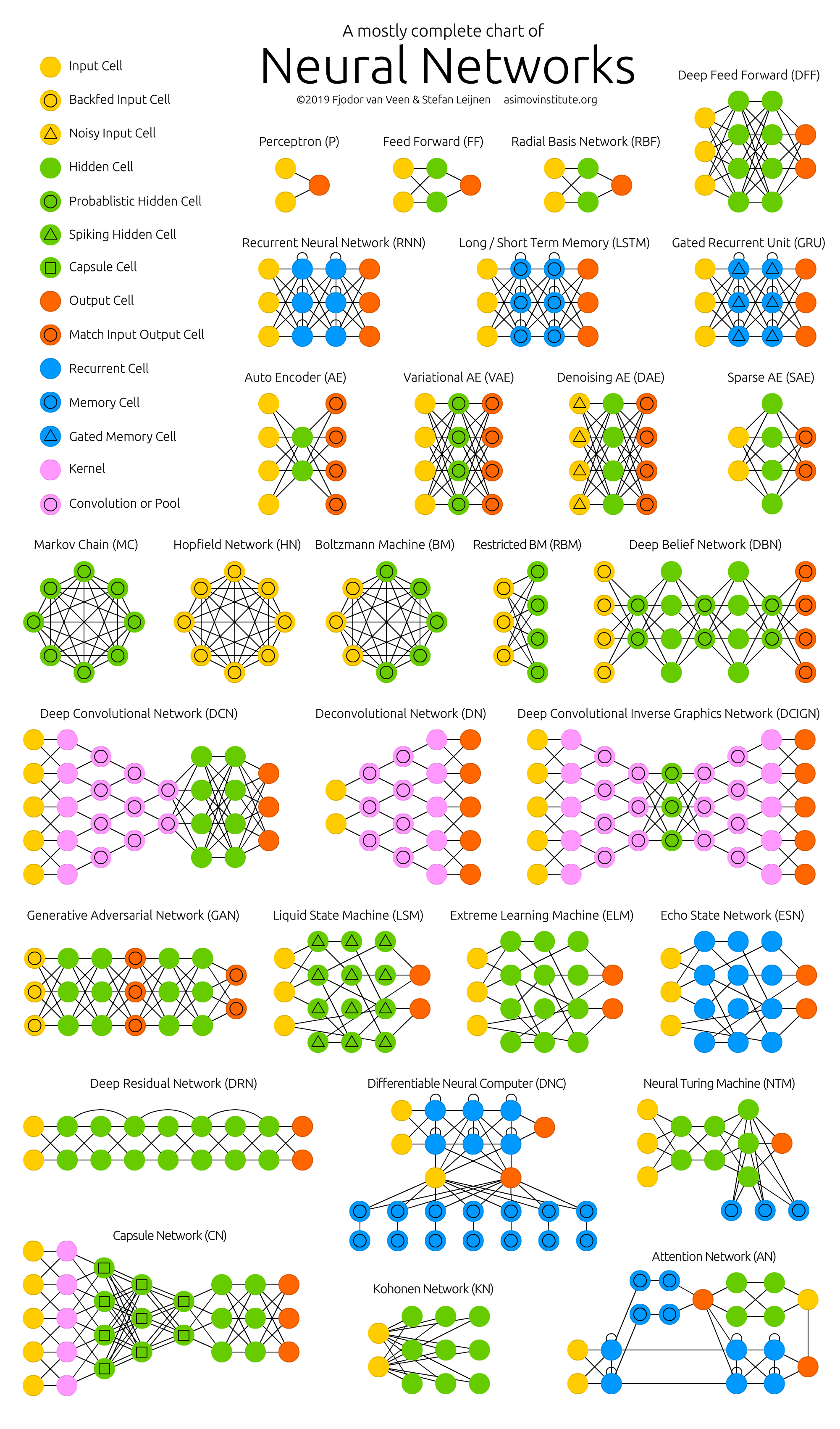 The Neural Network Zoo (download or get the poster).
One problem with drawing them as node maps: it doesn’t really show how they’re used. For example, variational autoencoders (VAE) may look just like autoencoders (AE), but the training process is actually quite different. The use-cases for trained networks differ even more, because VAEs are generators, where you insert noise to get a new sample. AEs, simply map whatever they get as input to the closest training sample they “remember”. I should add that this overview is in no way clarifying how each of the different node types work internally (but that’s a topic for another day).
It should be noted that while most of the abbreviations used are generally accepted, not all of them are. RNNs sometimes refer to recursive neural networks, but most of the time they refer to recurrent neural networks. That’s not the end of it though, in many places you’ll find RNN used as placeholder for any recurrent architecture, including LSTMs, GRUs and even the bidirectional variants. AEs suffer from a similar problem from time to time, where VAEs and DAEs and the like are called simply AEs. Many abbreviations also vary in the amount of “N”s to add at the end, because you could call it a convolutional neural network but also simply a convolutional network (resulting in CNN or CN).
Composing a complete list is practically impossible, as new architectures are invented all the time. Even if published it can still be quite challenging to find them even if you’re looking for them, or sometimes you just overlook some. So while this list may provide you with some insights into the world of AI, please, by no means take this list for being comprehensive; especially if you read this post long after it was written.
For each of the architectures depicted in the picture, I wrote a very, very brief description. You may find some of these to be useful if you’re quite familiar with some architectures, but you aren’t familiar with a particular one.

Feed forward neural networks (FF or FFNN) and perceptrons (P) are very straight forward, they feed information from the front to the back (input and output, respectively). Neural networks are often described as having layers, where each layer consists of either input, hidden or output cells in parallel. A layer alone never has connections and in general two adjacent layers are fully connected (every neuron form one layer to every neuron to another layer). The simplest somewhat practical network has two input cells and one output cell, which can be used to model logic gates. One usually trains FFNNs through back-propagation, giving the network paired datasets of “what goes in” and “what we want to have coming out”. This is called supervised learning, as opposed to unsupervised learning where we only give it input and let the network fill in the blanks. The error being back-propagated is often some variation of the difference between the input and the output (like MSE or just the linear difference). Given that the network has enough hidden neurons, it can theoretically always model the relationship between the input and output. Practically their use is a lot more limited but they are popularly combined with other networks to form new networks.
Rosenblatt, Frank. “The perceptron: a probabilistic model for information storage and organization in the brain.” Psychological review 65.6 (1958): 386.
Original Paper PDF

Radial basis function (RBF) networks are FFNNs with radial basis functions as activation functions. There’s nothing more to it. Doesn’t mean they don’t have their uses, but most FFNNs with other activation functions don’t get their own name. This mostly has to do with inventing them at the right time.
Broomhead, David S., and David Lowe. Radial basis functions, multi-variable functional interpolation and adaptive networks. No. RSRE-MEMO-4148. ROYAL SIGNALS AND RADAR ESTABLISHMENT MALVERN (UNITED KINGDOM), 1988.
Original Paper PDF

Recurrent neural networks (RNN) are FFNNs with a time twist: they are not stateless; they have connections between passes, connections through time. Neurons are fed information not just from the previous layer but also from themselves from the previous pass. This means that the order in which you feed the input and train the network matters: feeding it “milk” and then “cookies” may yield different results compared to feeding it “cookies” and then “milk”. One big problem with RNNs is the vanishing (or exploding) gradient problem where, depending on the activation functions used, information rapidly gets lost over time, just like very deep FFNNs lose information in depth. Intuitively this wouldn’t be much of a problem because these are just weights and not neuron states, but the weights through time is actually where the information from the past is stored; if the weight reaches a value of 0 or 1 000 000, the previous state won’t be very informative. RNNs can in principle be used in many fields as most forms of data that don’t actually have a timeline (i.e. unlike sound or video) can be represented as a sequence. A picture or a string of text can be fed one pixel or character at a time, so the time dependent weights are used for what came before in the sequence, not actually from what happened x seconds before. In general, recurrent networks are a good choice for advancing or completing information, such as autocompletion.
Elman, Jeffrey L. “Finding structure in time.” Cognitive science 14.2 (1990): 179-211.
Original Paper PDF

Long / short term memory (LSTM) networks try to combat the vanishing / exploding gradient problem by introducing gates and an explicitly defined memory cell. These are inspired mostly by circuitry, not so much biology. Each neuron has a memory cell and three gates: input, output and forget. The function of these gates is to safeguard the information by stopping or allowing the flow of it. The input gate determines how much of the information from the previous layer gets stored in the cell. The output layer takes the job on the other end and determines how much of the next layer gets to know about the state of this cell. The forget gate seems like an odd inclusion at first but sometimes it’s good to forget: if it’s learning a book and a new chapter begins, it may be necessary for the network to forget some characters from the previous chapter. LSTMs have been shown to be able to learn complex sequences, such as writing like Shakespeare or composing primitive music. Note that each of these gates has a weight to a cell in the previous neuron, so they typically require more resources to run.
Hochreiter, Sepp, and Jürgen Schmidhuber. “Long short-term memory.” Neural computation 9.8 (1997): 1735-1780.
Original Paper PDF

Gated recurrent units (GRU) are a slight variation on LSTMs. They have one less gate and are wired slightly differently: instead of an input, output and a forget gate, they have an update gate. This update gate determines both how much information to keep from the last state and how much information to let in from the previous layer. The reset gate functions much like the forget gate of an LSTM but it’s located slightly differently. They always send out their full state, they don’t have an output gate. In most cases, they function very similarly to LSTMs, with the biggest difference being that GRUs are slightly faster and easier to run (but also slightly less expressive). In practice these tend to cancel each other out, as you need a bigger network to regain some expressiveness which then in turn cancels out the performance benefits. In some cases where the extra expressiveness is not needed, GRUs can outperform LSTMs.
Chung, Junyoung, et al. “Empirical evaluation of gated recurrent neural networks on sequence modeling.” arXiv preprint arXiv:1412.3555 (2014).
Original Paper PDF
Bidirectional recurrent neural networks, bidirectional long / short term memory networks and bidirectional gated recurrent units (BiRNN, BiLSTM and BiGRU respectively) are not shown on the chart because they look exactly the same as their unidirectional counterparts. The difference is that these networks are not just connected to the past, but also to the future. As an example, unidirectional LSTMs might be trained to predict the word “fish” by being fed the letters one by one, where the recurrent connections through time remember the last value. A BiLSTM would also be fed the next letter in the sequence on the backward pass, giving it access to future information. This trains the network to fill in gaps instead of advancing information, so instead of expanding an image on the edge, it could fill a hole in the middle of an image.
Schuster, Mike, and Kuldip K. Paliwal. “Bidirectional recurrent neural networks.” IEEE Transactions on Signal Processing 45.11 (1997): 2673-2681.
Original Paper PDF

Autoencoders (AE) are somewhat similar to FFNNs as AEs are more like a different use of FFNNs than a fundamentally different architecture. The basic idea behind autoencoders is to encode information (as in compress, not encrypt) automatically, hence the name. The entire network always resembles an hourglass like shape, with smaller hidden layers than the input and output layers. AEs are also always symmetrical around the middle layer(s) (one or two depending on an even or odd amount of layers). The smallest layer(s) is|are almost always in the middle, the place where the information is most compressed (the chokepoint of the network). Everything up to the middle is called the encoding part, everything after the middle the decoding and the middle (surprise) the code. One can train them using backpropagation by feeding input and setting the error to be the difference between the input and what came out. AEs can be built symmetrically when it comes to weights as well, so the encoding weights are the same as the decoding weights.
Bourlard, Hervé, and Yves Kamp. “Auto-association by multilayer perceptrons and singular value decomposition.” Biological cybernetics 59.4-5 (1988): 291-294.
Original Paper PDF

Variational autoencoders (VAE) have the same architecture as AEs but are “taught” something else: an approximated probability distribution of the input samples. It’s a bit back to the roots as they are bit more closely related to BMs and RBMs. They do however rely on Bayesian mathematics regarding probabilistic inference and independence, as well as a re-parametrisation trick to achieve this different representation. The inference and independence parts make sense intuitively, but they rely on somewhat complex mathematics. The basics come down to this: take influence into account. If one thing happens in one place and something else happens somewhere else, they are not necessarily related. If they are not related, then the error propagation should consider that. This is a useful approach because neural networks are large graphs (in a way), so it helps if you can rule out influence from some nodes to other nodes as you dive into deeper layers.
Kingma, Diederik P., and Max Welling. “Auto-encoding variational bayes.” arXiv preprint arXiv:1312.6114 (2013).
Original Paper PDF

Denoising autoencoders (DAE) are AEs where we don’t feed just the input data, but we feed the input data with noise (like making an image more grainy). We compute the error the same way though, so the output of the network is compared to the original input without noise. This encourages the network not to learn details but broader features, as learning smaller features often turns out to be “wrong” due to it constantly changing with noise.
Vincent, Pascal, et al. “Extracting and composing robust features with denoising autoencoders.” Proceedings of the 25th international conference on Machine learning. ACM, 2008.
Original Paper PDF

Sparse autoencoders (SAE) are in a way the opposite of AEs. Instead of teaching a network to represent a bunch of information in less “space” or nodes, we try to encode information in more space. So instead of the network converging in the middle and then expanding back to the input size, we blow up the middle. These types of networks can be used to extract many small features from a dataset. If one were to train a SAE the same way as an AE, you would in almost all cases end up with a pretty useless identity network (as in what comes in is what comes out, without any transformation or decomposition). To prevent this, instead of feeding back the input, we feed back the input plus a sparsity driver. This sparsity driver can take the form of a threshold filter, where only a certain error is passed back and trained, the other error will be “irrelevant” for that pass and set to zero. In a way this resembles spiking neural networks, where not all neurons fire all the time (and points are scored for biological plausibility).
Marc’Aurelio Ranzato, Christopher Poultney, Sumit Chopra, and Yann LeCun. “Efficient learning of sparse representations with an energy-based model.” Proceedings of NIPS. 2007.
Original Paper PDF

Markov chains (MC or discrete time Markov Chain, DTMC) are kind of the predecessors to BMs and HNs. They can be understood as follows: from this node where I am now, what are the odds of me going to any of my neighbouring nodes? They are memoryless (i.e. Markov Property) which means that every state you end up in depends completely on the previous state. While not really a neural network, they do resemble neural networks and form the theoretical basis for BMs and HNs. MC aren’t always considered neural networks, as goes for BMs, RBMs and HNs. Markov chains aren’t always fully connected either.
Hayes, Brian. “First links in the Markov chain.” American Scientist 101.2 (2013): 252.
Original Paper PDF

A Hopfield network (HN) is a network where every neuron is connected to every other neuron; it is a completely entangled plate of spaghetti as even all the nodes function as everything. Each node is input before training, then hidden during training and output afterwards. The networks are trained by setting the value of the neurons to the desired pattern after which the weights can be computed. The weights do not change after this. Once trained for one or more patterns, the network will always converge to one of the learned patterns because the network is only stable in those states. Note that it does not always conform to the desired state (it’s not a magic black box sadly). It stabilises in part due to the total “energy” or “temperature” of the network being reduced incrementally during training. Each neuron has an activation threshold which scales to this temperature, which if surpassed by summing the input causes the neuron to take the form of one of two states (usually -1 or 1, sometimes 0 or 1). Updating the network can be done synchronously or more commonly one by one. If updated one by one, a fair random sequence is created to organise which cells update in what order (fair random being all options (n) occurring exactly once every n items). This is so you can tell when the network is stable (done converging), once every cell has been updated and none of them changed, the network is stable (annealed). These networks are often called associative memory because the converge to the most similar state as the input; if humans see half a table we can image the other half, this network will converge to a table if presented with half noise and half a table.
Hopfield, John J. “Neural networks and physical systems with emergent collective computational abilities.” Proceedings of the national academy of sciences 79.8 (1982): 2554-2558.
Original Paper PDF

Boltzmann machines (BM) are a lot like HNs, but: some neurons are marked as input neurons and others remain “hidden”. The input neurons become output neurons at the end of a full network update. It starts with random weights and learns through back-propagation, or more recently through contrastive divergence (a Markov chain is used to determine the gradients between two informational gains). Compared to a HN, the neurons mostly have binary activation patterns. As hinted by being trained by MCs, BMs are stochastic networks. The training and running process of a BM is fairly similar to a HN: one sets the input neurons to certain clamped values after which the network is set free (it doesn’t get a sock). While free the cells can get any value and we repetitively go back and forth between the input and hidden neurons. The activation is controlled by a global temperature value, which if lowered lowers the energy of the cells. This lower energy causes their activation patterns to stabilise. The network reaches an equilibrium given the right temperature.
Hinton, Geoffrey E., and Terrence J. Sejnowski. “Learning and releaming in Boltzmann machines.” Parallel distributed processing: Explorations in the microstructure of cognition 1 (1986): 282-317.
Original Paper PDF

Restricted Boltzmann machines (RBM) are remarkably similar to BMs (surprise) and therefore also similar to HNs. The biggest difference between BMs and RBMs is that RBMs are a better usable because they are more restricted. They don’t trigger-happily connect every neuron to every other neuron but only connect every different group of neurons to every other group, so no input neurons are directly connected to other input neurons and no hidden to hidden connections are made either. RBMs can be trained like FFNNs with a twist: instead of passing data forward and then back-propagating, you forward pass the data and then backward pass the data (back to the first layer). After that you train with forward-and-back-propagation.
Smolensky, Paul. Information processing in dynamical systems: Foundations of harmony theory. No. CU-CS-321-86. COLORADO UNIV AT BOULDER DEPT OF COMPUTER SCIENCE, 1986.
Original Paper PDF

Deep belief networks (DBN) is the name given to stacked architectures of mostly RBMs or VAEs. These networks have been shown to be effectively trainable stack by stack, where each AE or RBM only has to learn to encode the previous network. This technique is also known as greedy training, where greedy means making locally optimal solutions to get to a decent but possibly not optimal answer. DBNs can be trained through contrastive divergence or back-propagation and learn to represent the data as a probabilistic model, just like regular RBMs or VAEs. Once trained or converged to a (more) stable state through unsupervised learning, the model can be used to generate new data. If trained with contrastive divergence, it can even classify existing data because the neurons have been taught to look for different features.
Bengio, Yoshua, et al. “Greedy layer-wise training of deep networks.” Advances in neural information processing systems 19 (2007): 153.
Original Paper PDF

Convolutional neural networks (CNN or deep convolutional neural networks, DCNN) are quite different from most other networks. They are primarily used for image processing but can also be used for other types of input such as as audio. A typical use case for CNNs is where you feed the network images and the network classifies the data, e.g. it outputs “cat” if you give it a cat picture and “dog” when you give it a dog picture. CNNs tend to start with an input “scanner” which is not intended to parse all the training data at once. For example, to input an image of 200 x 200 pixels, you wouldn’t want a layer with 40 000 nodes. Rather, you create a scanning input layer of say 20 x 20 which you feed the first 20 x 20 pixels of the image (usually starting in the upper left corner). Once you passed that input (and possibly use it for training) you feed it the next 20 x 20 pixels: you move the scanner one pixel to the right. Note that one wouldn’t move the input 20 pixels (or whatever scanner width) over, you’re not dissecting the image into blocks of 20 x 20, but rather you’re crawling over it. This input data is then fed through convolutional layers instead of normal layers, where not all nodes are connected to all nodes. Each node only concerns itself with close neighbouring cells (how close depends on the implementation, but usually not more than a few). These convolutional layers also tend to shrink as they become deeper, mostly by easily divisible factors of the input (so 20 would probably go to a layer of 10 followed by a layer of 5). Powers of two are very commonly used here, as they can be divided cleanly and completely by definition: 32, 16, 8, 4, 2, 1. Besides these convolutional layers, they also often feature pooling layers. Pooling is a way to filter out details: a commonly found pooling technique is max pooling, where we take say 2 x 2 pixels and pass on the pixel with the most amount of red. To apply CNNs for audio, you basically feed the input audio waves and inch over the length of the clip, segment by segment. Real world implementations of CNNs often glue an FFNN to the end to further process the data, which allows for highly non-linear abstractions. These networks are called DCNNs but the names and abbreviations between these two are often used interchangeably.
LeCun, Yann, et al. “Gradient-based learning applied to document recognition.” Proceedings of the IEEE 86.11 (1998): 2278-2324.
Original Paper PDF

Deconvolutional networks (DN), also called inverse graphics networks (IGNs), are reversed convolutional neural networks. Imagine feeding a network the word “cat” and training it to produce cat-like pictures, by comparing what it generates to real pictures of cats. DNNs can be combined with FFNNs just like regular CNNs, but this is about the point where the line is drawn with coming up with new abbreviations. They may be referenced as deep deconvolutional neural networks, but you could argue that when you stick FFNNs to the back and the front of DNNs that you have yet another architecture which deserves a new name. Note that in most applications one wouldn’t actually feed text-like input to the network, more likely a binary classification input vector. Think <0, 1> being cat, <1, 0> being dog and <1, 1> being cat and dog. The pooling layers commonly found in CNNs are often replaced with similar inverse operations, mainly interpolation and extrapolation with biased assumptions (if a pooling layer uses max pooling, you can invent exclusively lower new data when reversing it).
Zeiler, Matthew D., et al. “Deconvolutional networks.” Computer Vision and Pattern Recognition (CVPR), 2010 IEEE Conference on. IEEE, 2010.
Original Paper PDF

Deep convolutional inverse graphics networks (DCIGN) have a somewhat misleading name, as they are actually VAEs but with CNNs and DNNs for the respective encoders and decoders. These networks attempt to model “features” in the encoding as probabilities, so that it can learn to produce a picture with a cat and a dog together, having only ever seen one of the two in separate pictures. Similarly, you could feed it a picture of a cat with your neighbours’ annoying dog on it, and ask it to remove the dog, without ever having done such an operation. Demo’s have shown that these networks can also learn to model complex transformations on images, such as changing the source of light or the rotation of a 3D object. These networks tend to be trained with back-propagation.
Kulkarni, Tejas D., et al. “Deep convolutional inverse graphics network.” Advances in Neural Information Processing Systems. 2015.
Original Paper PDF

Generative adversarial networks (GAN) are from a different breed of networks, they are twins: two networks working together. GANs consist of any two networks (although often a combination of FFs and CNNs), with one tasked to generate content and the other has to judge content. The discriminating network receives either training data or generated content from the generative network. How well the discriminating network was able to correctly predict the data source is then used as part of the error for the generating network. This creates a form of competition where the discriminator is getting better at distinguishing real data from generated data and the generator is learning to become less predictable to the discriminator. This works well in part because even quite complex noise-like patterns are eventually predictable but generated content similar in features to the input data is harder to learn to distinguish. GANs can be quite difficult to train, as you don’t just have to train two networks (either of which can pose it’s own problems) but their dynamics need to be balanced as well. If prediction or generation becomes to good compared to the other, a GAN won’t converge as there is intrinsic divergence.
Goodfellow, Ian, et al. “Generative adversarial nets.” Advances in Neural Information Processing Systems (2014).
Original Paper PDF

Liquid state machines (LSM) are similar soups, looking a lot like ESNs. The real difference is that LSMs are a type of spiking neural networks: sigmoid activations are replaced with threshold functions and each neuron is also an accumulating memory cell. So when updating a neuron, the value is not set to the sum of the neighbours, but rather added to itself. Once the threshold is reached, it releases its’ energy to other neurons. This creates a spiking like pattern, where nothing happens for a while until a threshold is suddenly reached.
Maass, Wolfgang, Thomas Natschläger, and Henry Markram. “Real-time computing without stable states: A new framework for neural computation based on perturbations.” Neural computation 14.11 (2002): 2531-2560.
Original Paper PDF

Extreme learning machines (ELM) are basically FFNNs but with random connections. They look very similar to LSMs and ESNs, but they are not recurrent nor spiking. They also do not use backpropagation. Instead, they start with random weights and train the weights in a single step according to the least-squares fit (lowest error across all functions). This results in a much less expressive network but it’s also much faster than backpropagation.
Huang, Guang-Bin, et al. “Extreme learning machine: Theory and applications.” Neurocomputing 70.1-3 (2006): 489-501.
Original Paper PDF

Echo state networks (ESN) are yet another different type of (recurrent) network. This one sets itself apart from others by having random connections between the neurons (i.e. not organised into neat sets of layers), and they are trained differently. Instead of feeding input and back-propagating the error, we feed the input, forward it and update the neurons for a while, and observe the output over time. The input and the output layers have a slightly unconventional role as the input layer is used to prime the network and the output layer acts as an observer of the activation patterns that unfold over time. During training, only the connections between the observer and the (soup of) hidden units are changed.
Jaeger, Herbert, and Harald Haas. “Harnessing nonlinearity: Predicting chaotic systems and saving energy in wireless communication.” science 304.5667 (2004): 78-80.
Original Paper PDF

Deep residual networks (DRN) are very deep FFNNs with extra connections passing input from one layer to a later layer (often 2 to 5 layers) as well as the next layer. Instead of trying to find a solution for mapping some input to some output across say 5 layers, the network is enforced to learn to map some input to some output + some input. Basically, it adds an identity to the solution, carrying the older input over and serving it freshly to a later layer. It has been shown that these networks are very effective at learning patterns up to 150 layers deep, much more than the regular 2 to 5 layers one could expect to train. However, it has been proven that these networks are in essence just RNNs without the explicit time based construction and they’re often compared to LSTMs without gates.
He, Kaiming, et al. “Deep residual learning for image recognition.” arXiv preprint arXiv:1512.03385 (2015).
Original Paper PDF

Neural Turing machines (NTM) can be understood as an abstraction of LSTMs and an attempt to un-black-box neural networks (and give us some insight in what is going on in there). Instead of coding a memory cell directly into a neuron, the memory is separated. It’s an attempt to combine the efficiency and permanency of regular digital storage and the efficiency and expressive power of neural networks. The idea is to have a content-addressable memory bank and a neural network that can read and write from it. The “Turing” in Neural Turing Machines comes from them being Turing complete: the ability to read and write and change state based on what it reads means it can represent anything a Universal Turing Machine can represent.
Graves, Alex, Greg Wayne, and Ivo Danihelka. “Neural turing machines.” arXiv preprint arXiv:1410.5401 (2014).
Original Paper PDF

Differentiable Neural Computers (DNC) are enhanced Neural Turing Machines with scalable memory, inspired by how memories are stored by the human hippocampus. The idea is to take the classical Von Neumann computer architecture and replace the CPU with an RNN, which learns when and what to read from the RAM. Besides having a large bank of numbers as memory (which may be resized without retraining the RNN). The DNC also has three attention mechanisms. These mechanisms allow the RNN to query the similarity of a bit of input to the memory’s entries, the temporal relationship between any two entries in memory, and whether a memory entry was recently updated – which makes it less likely to be overwritten when there’s no empty memory available.
Graves, Alex, et al. “Hybrid computing using a neural network with dynamic external memory.” Nature 538 (2016): 471-476.
Original Paper PDF

Capsule Networks (CapsNet) are biology inspired alternatives to pooling, where neurons are connected with multiple weights (a vector) instead of just one weight (a scalar). This allows neurons to transfer more information than simply which feature was detected, such as where a feature is in the picture or what colour and orientation it has. The learning process involves a local form of Hebbian learning that values correct predictions of output in the next layer.
Sabour, Sara, Frosst, Nicholas, and Hinton, G. E. “Dynamic Routing Between Capsules.” In Advances in neural information processing systems (2017): 3856-3866.
Original Paper PDF

Kohonen networks (KN, also self organising (feature) map, SOM, SOFM) utilise competitive learning to classify data without supervision. Input is presented to the network, after which the network assesses which of its neurons most closely match that input. These neurons are then adjusted to match the input even better, dragging along their neighbours in the process. How much the neighbours are moved depends on the distance of the neighbours to the best matching units.
Kohonen, Teuvo. “Self-organized formation of topologically correct feature maps.” Biological cybernetics 43.1 (1982): 59-69.
Original Paper PDF

Attention networks (AN) can be considered a class of networks, which includes the Transformer architecture. They use an attention mechanism to combat information decay by separately storing previous network states and switching attention between the states. The hidden states of each iteration in the encoding layers are stored in memory cells. The decoding layers are connected to the encoding layers, but it also receives data from the memory cells filtered by an attention context. This filtering step adds context for the decoding layers stressing the importance of particular features. The attention network producing this context is trained using the error signal from the output of decoding layer. Moreover, the attention context can be visualized giving valuable insight into which input features correspond with what output features.
Jaderberg, Max, et al. “Spatial Transformer Networks.” In Advances in neural information processing systems (2015): 2017-2025.
Original Paper PDF
Follow us on twitter for future updates and posts. We welcome comments and feedback, and thank you for reading!
[Update 22 April 2019] Included Capsule Networks, Differentiable Neural Computers and Attention Networks to the Neural Network Zoo; Support Vector Machines are removed; updated links to original articles. The previous version of this post can be found here .
Van Veen, F. & Leijnen, S. (2019). The Neural Network Zoo. Retrieved from https://www.asimovinstitute.org/neural-network-zoo
how about recursive neural networks?
Interesting, another branch of networks. Will definitely incorporate them in a potential follow up post!
Awesome. Minor correction regarding Boltzmann machines. “Compared to a HN, the neurons also sometimes have binary activation patterns but at other times they are stochastic”. The units are always stochastic, and usually also binary. But there are variations where units are instead Gaussian, binomial, etc.
Good stuff. Thank you for your feedback!
I don’t understand why in Markov chains you have a fully-connected graph. It should be either a chain, or a generalized “chain” where previous m nodes have edges to current node (if we’re talking about m-order markov chains)
Thank you for your feedback! When you say chain, you mean something like this? http://blogs.canisius.edu/mathblog/wp-content/uploads/sites/31/2013/02/markovchainpic3.png
Or more like this? http://1.bp.blogspot.com/-uLVbBbNTDTI/TbWSnEa4ZpI/AAAAAAAAABY/XYrTCXRhSkQ/s1600/markovchain.png
Note that all architectures have a rather finite representation here. As pointed out elsewhere, the DAEs often have a complete or overcomplete hidden layer, but not always. Most examples I can find are either arbitrary chains or fully connected graphs.
Yes, something like this but without loops. Basically a bunch of probabilistic cells (if you make them hidden, you get a HMM) chained in a linear way.
Hmm, will take that into consideration. The cells themselves are not probabilistic though, the connections between them are. I’m considering giving a few example networks for some architectures, especially the ones that vary greatly like this one.
Now that you mention that, I’m confused as to what kind of Markov chain the chart has.
Cool! I think you could give the denoising autoencoder a higher-dimensional hidden layer since it doesn’t need a bottleneck.
From what I understand, DAEs are simply AEs but used differently, which themselves are just symmetric FFNNs used differently. It is true that DAEs are often either complete or overcomplete, since overcomplete AEs usually learn identity; this is what DAEs are trying to prevent. The size restrictions are rarely explicitly defined though. Thank you for reading!
This reply is a hidden layer
Excellent work!
Could you please enhance the article by adding and presenting the Hidden Markov models using exactly the same approach ? That would be very enlightening, and I am very curious to read your explanation. Thank you
Working on it [:
Awesome! Could you also add some references for each network?
I’d love to, if I can find the time [:
Awesome work! Btw, should the middle neurons in the Deep convolutional inverse graphics networks (DCIGN) be probabilistic hidden cells?
Yes. Good observation, will correct!
Very nice summary!
From the pictures of the denoising autoencoder and the variational autoencoder, it looks like they also have to compress the data (since the hidden layer has fewer elements than the input and output layers), just the ordinary autoencoder. Is that the case?
Also, is there some specific name for the ordinary autoencoder to let people know that you are talking about an autoencoder that compresses the data? Perhaps “compressive autoencoder”? To me, the term “autoencoder” includes all kinds of autoencoders, i.e. also denoising, variational and sparse autoencoders, not just “compressive” (?) autoencoders. (So to me it feels a bit wrong to talk about “autoencoders” like all of them compress the data.)
A common problem with the networks. RNN stands for either recurrent NN or recursive NN. Worse yet, people use RNN to indicate LSTM, GRU, BiGRU and BiLSTM. And no, there is no name for that.
And yes, a problem with this “one shot” representation is that you cannot capture all uses. AE, VAE, SAE and DAE are all autoencoders, each of which somehow tries to reconstruct their input. Only SAEs almost always have an overcomplete code (more hidden neurons than input / output), but the others can have compressed, complete or overcomplete codes.
Thank you for your feedback!
Amazing. What software did you used to plot these figures ? Cheers !
I drew them in Adobe Animate, they’re not plots. Yes it was a lot of work to draw the lines.
Therefore they look really amazing! Would it be possible to publish the images as vector? Maybe in SVG or some other format? I would like to use them in my Master thesis. Of course I would cite you 🙂
Thanks, please do! I have a poster link of the whole thing which is 8k resolution, best I can do for now sorry.
Could another version of the poster be produced with the descriptions incorporated?
I’d love to hang one somewhere to keep them fresh in my memory (and also because the art work is lovely).
Wow great work on the summary and high quality images! May I also cite you in my thesis and use a snippet of the 8K poster for demonstrative purposes? Thanks for the article, ANNs are less confusing after reading it.)
Never thought of SVMs as a network, though they can be used that way. This seems to be a different take on SVMs than I’ve heard before.
Absolutely the best article and classification I have read in 10 years. Clearly written, easily understood. Points anyone reading to research those areas applicable to their problem set.
One of the most useful and comprehensive posts I’ve seen in a while. Very nicely done 🙂
I’m the creator of Deeplearning.TV on YouTube. If you would like to follow this up with a series of videos explaining this, I would be honored to collaborate with you 🙂
Very nice work!
I have a question,why svm could be seen as as a 3 level network,and the input cells are not full connected to the first hiden level, what’s that mean?
The idea behind deeper SVMs is that they allow for classification tasks more complex than binary. Usually it would just be the directly one-to-one connected stuff as seen in the first layer. It’s set up like that because each neuron in the input represents a point in the possibility space, and the network tries to separate the inputs with a margin as large as possible.
Thanks for your quick reply!
Could you please give me some reference papers about
svm-network, i ‘m interested in this research how neural network could union these algorthims.
Embedding SVMs in the framework of neural networks is an intriguing idea. I’d love to read more about this, too. Is there a paper on this or where does this idea come from?
Can you eventually give a link to a high resolution image of these networks? I was thinking about getting a poster printed for myself.
Cool! See the bottom of the post.
Nice job, summarizing and representing all of these! One observation regarding GANs is that the discriminator, as originally conceived, has only two output neurons (whether the sample passed to it came from the true distribution or from the generated one). The corresponding graphic shows three.
Yes. On it. Although you could also make do with one, I think I’ll draw it with two. Thank you!
You’re right! The discriminator does actually a regression on that one decision so one output is indeed more precise (although having two neurons drawn looks more representative to me)
Fixed it.
Hi, thanks for the very nice visualization! A common mistake with RNNs is to not connect neurons within the same layer. While each LSTM neuron has its own hidden state, its output feeds back to all neurons in the current layer. The mistake also appears here.
Keen eye! Forgot to draw the lines, but very aware of the fine workings. It will make it a spiderweb of lines, but eh [:
[UPDATE] fixed
Are you excellent images available for reuse under a particular license? Do you have an attribution policy?
As long as you mention the author and link to the Asimov Institute, use them however and wherever you like!
If you look closely, you’ll find only completely blind people will not be able to read the image. There are slight lines on the circle edges with unique patterns for each of the five different colours.
If I turn off color blind enhancement, I can technically tell input and hidden cells apart, especially if they are adjacent. In practice, I was using a program which tells me the color under the cursor to be sure. In the normal view, it’s as if you used coins differing only in the date minted, instead of gold and green. I don’t want to give you a hard time, I just noticed that you probably spent a lot of time on the graphics, and I thought I’d share what I can actually see. No reply necessary.
Hey , nice coverage ! Even wasn’t aware of a couple of architectures myself. BTW, you can integrate Fully Convolutional Nets (like FCN, U-Net, V-Nets ) etc. Also Deep Recurrent Convolutional Nets (DRCNs) might be a good idea to give an idea of merging of RNNs & CNNs
Will look into those. May have a to draw a line at some point, I cannot add all the possible permutations of all different cells. At some point someone may find a use for deep residual convolutional long short term memory echo state networks [:
Thank you for pointing them out though!
This is beautiful. Thank you so much.
Hi, could you add horizontal line between each explanation please. I get confused easily.
Thanks for the wonderful explanation
Good idea, thank you!
Good job! Thanks a lot.
Hi
that’s very nice
Thank you so much
if I want to use some of these information in my paper, how can cited?
I’d strongly recommend citing original papers, but feel free to use the images depicted here. Conventional citation methods should suffice just fine. Thank you for your interest!
Hi, great post, just a question. Doesn’t the number of outputs in a Kohonen Network should be 2 and the input N? Because those networks help you mapping multidimensional data into (x,y) coordinates for visualization, if I’m wrong, please correct me. And Kohonen networks help in dimensionality reduction, your input data should be multidimensional and it’s mapped to one or two dimensions.
https://www.cs.bham.ac.uk/~jlw/sem2a2/Web/Kohonen.htm
I think it’s a matter of choice, I see both representations frequently. As far as I understand it, the output you get is just one of the inputs. https://www.google.nl/search?q=kohonen+network&source=lnms&tbm=isch&sa=X&ved=0ahUKEwjUkrn9wJnPAhWiQJoKHZKwDZ4Q_AUICCgB&biw=1345&bih=1099&dpr=2#imgrc=_
Traditional Kohonen nets has k inputs and j processing nodes (outputs). It is a Competitive learning type of network with one layer (if we ignore the input vector). The output nodes (processing nodes) are traditionally mapped in 2D to reflect the topology in the input data (say, pixels in an image).
SVM is not implemented using neural networks. This is a beast from another zoo…
I know, that’s why I made a note of it. I included them because you can represent them as a network and they are used in machine learning applications [:
Hey there,
Thanks for the post. I’ve attempted to convert this into flashcards. It’s incredibly rough and wordy at the moment, but I will refine this over time. I am also still searching for definitions for your cell structures (backfed input cell, memory cell, etc.)
It’s available here: https://quizlet.com/152146730/neural-network-zoo-flash-cards/
My objectives are twofold:
1) I wanted to make sure you were okay with me retrofitting your work like this.
2) I was hoping you’d be able to help me fill in some of the blanks (literally and figuratively). I have tried to copy your blog post, but as I refine and explore, I’d love to have your input and notes to help inform its direction.
If you’re interested / want me to take it down, please let me know on here or via email.
Sure thing, cool project! Leave a note somewhere to the Asimov Institute and my name and I’m happy [:
I may do a follow up post explaining the different cells. They’re not official names, I just made them up. If you want to move forward quickly I’d recommend looking up the original papers; I’m confident you’ll be able to figure out why I gave the cells their names if you completely understand the networks and their uses. If you think of better names for the different cells, let me know!
If you have very specific questions, feel free to mail them to me, I can probably answer them relatively quickly.
Curious why there;’s no mention of network-in-network, the basis for GoogLeNet Inception
I would argue it;’s not curious at all, I simply overlooked it like some others! Thank you for pointing it out though, I will include it in the update!
This is pretty awesome. 🙂 I think that a great educational enhancement to this would be cite the original papers that introduced the associated network. Be a great way to introduce people learning to both the higher order concepts and the literature.
Coming soon… And thank you very much!
Extremely cool review. Short, simple, informative, contains references to original papers. Thank you very much!
I am stuned by all thé possibilités offered by ANN. I started to learn just few months ago and I am 60 ! So many thanks to you to have written superb articles ! Guy from Paris
Hello! would you please clarify, are the coloured discs cells within a neuron, and their network is an architecture within a neuron or how is it organised exactly? Thank you very much.
Each “disc” or circle represents a singular artificial neurone, the architecture is mostly the types of neurones used and how they’re connected. It’s also a little bit how they’re used, as some different neurones are really the same neurones but used in a different way (take noisy inputs and backfed outputs). Each connection represents a connection between two cells, simulating a neurite in a way.
Hey,
really nice post ! I’ve yet another suggestion for an additional network^^ :
It’s kind of an improved version of the echo state network where the crucial point is that they feed back the erroneous output back into the network. The first paper is this here: http://neurotheory.columbia.edu/Larry/SussilloNeuron09.pdf
They also managed to make the training work by changing the weights IN the network. Maybe you can just add it as more information for the echo state networks. There are several follow up papers on Larry Abbotts webpage where the link is from but I don’t know them (yet).
Thank you for your comment, cool findings. I will look into those; I may add them to the follow up post.
This is very good job. I would suggest where is the origin (perceptron) and make simple phylogenetic tree. Because here is Zoo.
Many thanks for this site.
Excellent work..Thank you so much. When we will see the other architectures?
Extreme Learning Machines don’t use backpropagation, they are random projections + a linear model.
Will look into it. Thanks for pointing it out!
It would be great if you could add the dynamics of each type of cell.
You should think about selling the summary figure as a poster.
Thanks for the suggestion, but I prefer to keep it as informative. If I end the post with a link to a webshop people will might see the whole thing as an ad.
Would love to see Contractive AEs in here
I have never seen SVMs classified as neural networks. The paper does call them support vector _networks_ and does compare/contrast them to perceptrons, but I still think it’s a fundamentally different approach to learning. It’s not connectivist.
Where is Helmholtz machine ?
Your Zoo is very beautiful and it is difficult to make it more beautiful. I was wondering whether we can add two more information to each network. One is weight constraints on each network and other is learning algorithm of each algorithm. I think your Zoo will become a little more beautiful. For learning algorithm, we may add another legend and place bars of different color under each network depicting what kind of learning algorithms may be used in each network. I could not figure out how the weight constrained information can be fitted artistically into this scheme. Maybe others can pitch in.
Just another question out of curiosity: which one of the neural networks presented here is nearest to an NMDA receptor?
Just asking because of this article:
http://journal.frontiersin.org/article/10.3389/fnsys.2016.00095/full
I reckon a combination of FF and possibly ELM. Sounds like a large deep FF network but with permanent learned dropout in the deeper layers. Interesting!
Great article, I keep sharing it with friends and colleagues, looking forward to follow-up post with the new architectures.
You mention demos of DCIGNs using more complex transformations, any way to get a link to one or at least the name of the researcher who did it.
Thank you! The original paper includes examples of rotation I believe.
Unfortunately, you forgot to mention all the family of Weightless Neural Systems.
Have a look at them, they are really interesting and powerful.
Massimo
Amazing, thank you.
Wonderful work! I would add “cascade correlation” ANNs, by Fahlman and Lebiere (1989). The cascade correlation learning architecture is:
“””
Cascade-Correlation begins with a minimal network, then automatically trains and adds new hidden units one by one, creating a multi-layer structure. Once a new hidden unit has been added to the network, its input-side weights are frozen. This unit then becomes a permanent feature-detector in the network, available for producing outputs or for creating other, more complex feature detectors.
“””
You could say that is a meta-algorithm, and a generative architecture. It adds hidden neurons as required by the task at hand. I know of two versions, Cascade-Correlation and recurrent Cascade-Correlation.
Primary source: Fahlman, S. E., & Lebiere, C. (1989). The cascade-correlation learning architecture.
Really great article. I just finished this semester’s course in Neural Nets and feel this NN Zoo perhaps lacks a few networks;
In competitive learning; Standard Competitive network and Lateral Inhibition Net. You included Kohonen SOM, so that’s nice. Further we have the Growing Hiearchical SOM (GHSOM) & variations of it.
Further; the Counter-propagation network is nice; a combo of Competitive/Kohonen layer & a feed forward layer, iirc, very practical (supervised learning on top of self-organized learning).
In associative memory nets there is also the Associatron and Bi-directional Associative Memory net (BAM), and nummerus modifications (IEEE has some articles, i.e. for PBHAM).
We also have the Cognitron and Neocognitron which were developed for rotation-invariant recognition of visual patterns.
Lastly there are the Generative Advisarial Networks, meant more for generating data than classifying, iirc (there is also the patented “Creativity machine”/”Imagination Engine” by Stephen Thaler).
Thanks again. 🙂
Forgot to say I like comprehensive overviews or lists, that is mostly why I mentioned these networks here.
Haven’t read the whole thing, but the graphics used are so aesthetically pleasing, that I simply fell in love with it. Thanks mate
Great post. Thanks
Great resource 🙂
Small comment: LSTM paper’s link does not work anymore 🙁
Are there any semi supervised NN? If it would be nice to add info on them.
It would be very convenient to make the keys/legend remain close to each graphical explanation !
Wow… you are a boss!
Can You add please the Spike NN, Boolean NN anf Fuzzy NN
Great article
Awesome work! I have started using it as a handy deep learning cookbook!
Hey, if you read this, please consider keeping the legend on the side as we scroll. I kept having to go back up to check the purpose of the nodes. Great article!
Minor nit. If you update the article, please consider stating that DCGAN stands for Deep Convolutional Generative Adversarial Networks
Very nice summary of the various structures. Would it be possible to reuse some of the pictures for an (academic) presentation, giving proper credits?
Good Job. The clean, precise and one of the best description.
Thanks a lot !
Hello,
Thank you for this great work!
I think it would be better to use arrows (when necessary) to indicate the stream of information between neurons. For instance, it could be helpful in order to distinguish between a deep feedforward network and and RBM.
Again, great job!
This post is awesome but needs some updates. There are lots of networks that need to be included.
This is an awesome initiative, giving an overview of models of neural nets out there, referencing original papers. Now, a nice squel could be a material covering methodology of training and approach used in hand-picked applications (e.g. AlphaGo).
Thank you very much!
Would it make sense to put some pseudo-code or Tensorflow code snippets along with the models to better illustrate how to setup a test?
Thank you for the comprehensive survey! This is very useful. I was wondering if you could also add a section on “Continuous-time recurrent neural networks” (CTRNN) which are often using the cognitive sciences? https://en.wikipedia.org/wiki/Recurrent_neural_network#Continuous-time
Thanks!
[…] Neural Networks Cheat Sheet: https://www.asimovinstitute.org/neural-network-zoo/ […]
Really nice work
[…] The Neural Network Zoo: https://www.asimovinstitute.org/neural-network-zoo/ […]
Its a good review of the networks. I would suggest extending the article with other deep learning frameworks available like resnet, densenet, vgg, inception, googlenet etc along with the fine-tuning concepts.
[…] The Neural Network Zoo (cheat sheet of nn architectures) […]
[…] second resource shared by Stephen is Fjodor Van Veen’s (2016) Neural Network Zoo. In his post Fjodor shares a “mostly complete chart of Neural […]
[…] There are many more curiosities and things to learn about the Neural Network Zoo. If that’s something that would make you more interested in Neural Networks and their intrinsic details, you can find it all in their own blog post here: https://www.asimovinstitute.org/neural-network-zoo/. […]
[…] Source: The Asimov Institute […]
[…] The first parameter defines the theme of node. For a neural network node (theme start with ‘nn.’), its style refers from Neural Network Zoo Page。 […]
[…] O’Reilly Media, 2017 S. Raschka et al. Deeper Insights into Machine Learning. Packt, 2016 https://www.asimovinstitute.org/neural-network-zoo/ https://www.microsoft.com/en-us/research/wp-content/uploads/2012/01/tricks-2012.pdf […]
[…] – LSTMネットワークの概要 – わかるLSTM ~ 最近の動向と共に – The Neural Network Zoo -> 全結合層や、CNN, […]
[…] the network right is the big part of the whole thing, that’s how it look). Sources like The Neural Network Zoo by the Asimov Institute, which shows different networks for different kinds of […]
[…] of neural networks and found some great resources. The Asimov Institute’s Neural Network Zoo (link), and Piotr Midgał’s very insightful paper on medium about the value of visualizing in […]
[…] There are many more curiosities and things to learn about the Neural Network Zoo. If that’s something that would make you more interested in Neural Networks and their intrinsic details, you can find it all in their own blog post here: https://www.asimovinstitute.org/neural-network-zoo/. […]
[…] the zoo of neural networks https://www.asimovinstitute.org/neural-network-zoo/ […]
[…] Exemplo de uma rede neural profunda. Fonte: The Asimov Institute […]
Nice zoo! Your description of SVMs is a little misleading – linear SVMs place a line, plane, or hyperplane to divide the two classes of data. They can use arbitrarily high dimensions, without kernels. The kernel trick is used to convert linear SVMs into non-linear SVMs. The kernel effectively distorts space, so that a linear SVM in the distorted space can now separate the data. The linear hyperplane can be thought of as a non-linear surface in the original (pre-distorted) space. Hope that clarifies things a little!
This is fantastic. Would it be possible to include the Winnow (version 2 if possible) Neural Network?
[…] Fig. 4. Tipos de Redes Neuronales. Tomada de The Asimov Institute. […]
[…] https://www.asimovinstitute.org/neural-network-zoo/ […]
[…] are many more network architectures in the wild. I recommend a good article called Neural Network Zoo, where almost all types of neural networks are collected and briefly […]
There are quite some things that are missing or just incorrect in these descriptions. For example in Convolutional Neural Networks, the kernel example size is 20×20, which is never used (only odd numbers, and even then most of the time only 3×3/5×5). These kernel sizes may reduce the size of the input, depends on if you use valid or same convolutions. And even if you use valid convolutions (same convolution doesn’t shrink the input) the size is only reduced by (kernel_width-1)/2, not by a factor of 2. The reduction by a factor of 2 is done by the pooling layers.
A well-known example for this can be seen in the U-net paper (https://arxiv.org/pdf/1505.04597.pdf) where the input size is 572×572, and after one convolutional layer the size is 570×570. Only the pooling layers reduce the size by 2 (can also be circumvented if input size isn’t that large with shift and stitch, but is computationally expensive.
Source: Master Data Science student that had to implement almost all architectures displayed above
Please correct the link from: http://cioslab.vcu.edu/alg/Visualize/kohonen-82.pdf to http://www.cnbc.cmu.edu/~tai/nc19journalclubs/Kohonen1982_Article_Self-organizedFormationOfTopol.pdf